Two Dimensional Weighting Function Example With an Ice Cloud
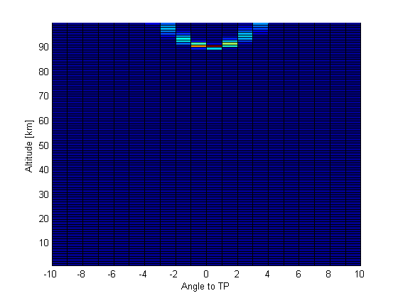
Here we calculate a two dimensional weighting function (angle along the line of sight, altitude) for a mesospheric ice cloud modeled by a Mie scattering code.
Matlab Version
engine = ISKEngine('HR');

% Background pressure
background = ISKClimatology('MSIS90');
rayleigh = ISKOpticalProperty('Rayleigh');
engine.AddSpecies('SKCLIMATOLOGY_AIRNUMBERDENSITY_CM3', background, rayleigh);

% Line of sight at ~89 km
mjd = 52385.25699403233;
look = [ 0.3181478 , -0.73086314, -0.60383859];
obs = [ 1707775.92848947, -1161098.50600522,  6655045.82625865];

engine.AddLineOfSight(mjd, obs, look);
engine.SetAlbedo(0.3);
engine.SetWavelengths([350]);

% MIEAEROSOL_WATER can also be used.  If switched to water remember to
% switch SKCLIMATOLOGY_AEROSOLICE_CM3 to SKCLIMATOLOGY_AEROSOLWATER_CM3
% below as well
ice = ISKOpticalProperty('MIEAEROSOL_ICE');

% Particle size could also be made two dimensional using the plane
% climatology as is done below
particle_size = ISKClimatology('USERDEFINED_PROFILE');
particle_size.SetProperty('Heights', [0, 100000]);
particle_size.SetPropertyUserDefined('SKCLIMATOLOGY_LOGNORMAL_MODERADIUS_MICRONS', [0.08, 0.08]);
particle_size.SetPropertyUserDefined('SKCLIMATOLOGY_LOGNORMAL_MODEWIDTH', [1.2, 1.2]);

% Two dimensional climatology
ice_climatology = ISKClimatology('USERDEFINED_PROFILE_PLANE');

% We have to define the plane that the climatology is specified in
geodetic = ISKGeodetic();
geodetic.SetLocationFromTangentPoint(obs, look);
tangent_point = geodetic.GetLocationXYZ();

reference = tangent_point / norm(tangent_point);
normal = cross(look, reference);
normal = normal' / norm(normal);

ice_climatology.SetProperty('normalandreference', [normal; reference]);

% Values in the two dimensional climatology are indexed by an angle and an
% altitude.  The angle is within the plane defined by the normal vector
% above, with the reference vector (the tangent point here) being 0
% degrees.  With the above definitions negative angles will be towards the
% observer and positive angles away from the observer

% Constant ice layer from 88 km to 92 km with no angular variation and
% number density 1/cm^3
altitudes = 88000:1000:92000;
angles = -10:10;
numden = ones(length(altitudes), length(angles));

ice_climatology.SetProperty('Heights', altitudes);
ice_climatology.SetProperty('Angles', angles);
ice_climatology.SetPropertyUserDefined('SKCLIMATOLOGY_AEROSOLICE_CM3', numden);

ice.SetProperty('SetParticleSizeClimatology', particle_size);

engine.AddSpecies('SKCLIMATOLOGY_AEROSOLICE_CM3', ice_climatology, ice);

% Turn on two dimensional mode in SASKTRAN
engine.SetProperty('opticaltabletype', 2);

% Tell SASKTRAN to calculate weighting functions for the ice species
engine.SetProperty('wfspecies', ice);

% and in two dimensions (altitude, angle in the plane)
engine.SetProperty('calcwf', 3);

% Do the calculation on the same grid that the ice climatology is defined
% on
engine.SetProperty('opticalanglegrid', angles);

% Also define the two dimensional plane within SASKTRAN
engine.SetProperty('opticalnormalandreference', [normal; reference]);

% Calculate the radiance and get the weighting functions
[ok, radiance] = engine.CalculateRadiance();
[ok, wf] = engine.GetWeightingFunctions();

% wf is (wavelength x lines of sight x atmospheric grid cells)
% only 1 wavelength and 1 line of sight
wf = squeeze(wf);
% wf is is now 2100x1, this is 100 altitudes (0.5:99.5) and 21 angles
wf = reshape(wf, 100, length(angles));
pcolor(angles,0.5:99.5, wf)
xlabel('Angle to TP');
ylabel('Altitude [km]');