Changing the Linear Components
Here we calculate trends using the SAGE II/OSIRIS/OMPS-LP Dataset. Trends are calculated in the following ways
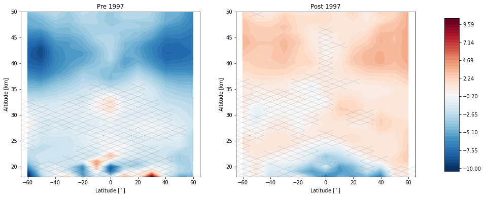
With two linear terms that have a join point at 1997.
Same as above but with the join point changed to 2000
By fitting ozone anomalies without any linear component, and then fitting the residuals to a linear term
Using two orthogonal forms of the EESC
Start with some imports and loading in the data
[2]:
import xarray as xr
import numpy as np
from LOTUS_regression.regression import regress_all_bins
from LOTUS_regression.predictors import load_data
import LOTUS_regression.predictors.download as download
import LOTUS_regression.plotting.trends as trends
import matplotlib.pyplot as plt
from datetime import datetime
import time
[3]:
MERGED_FILE = r'/media/users/data/LOTUS/S2_OS_OMPS/MERGED_LOTUS.nc'

mzm_data = xr.open_dataset(MERGED_FILE, engine='netcdf4')
We have our default set of predictors which contains linear terms joining at 1997
[4]:
predictors = load_data('pred_baseline_pwlt.csv').to_period('M')

print(predictors.columns)
Index(['enso', 'solar', 'qboA', 'qboB', 'aod', 'linear_pre', 'linear_post',
       'constant'],
      dtype='object')
And our default set of trends
[5]:
results = regress_all_bins(predictors, mzm_data['relative_anomaly'], tolerance=0.1)

# Convert to ~ percent
results *= 100

trends.pre_post_with_confidence(results, x='mean_latitude', y='altitude', ylim=(18, 50), log_y=False, figsize=(16, 6),
                                x_label='Latitude [$^\circ$]', y_label='Altitude [km]', pre_title='Pre 1997',
                                post_title='Post 1997')
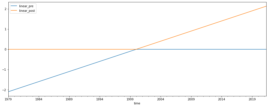
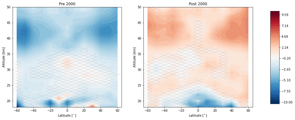
Now we change our inflection point in the linear trend to 2000 instead of 1997, and repeat the analysis
[6]:
predictors[['linear_pre', 'linear_post']] = download.load_linear(inflection=2000)[['pre','post']]

predictors[['linear_pre', 'linear_post']].plot(figsize=(16, 6))
[6]:
<AxesSubplot:xlabel='time'>
[7]:
results = regress_all_bins(predictors, mzm_data['relative_anomaly'], tolerance=0.1)

# Convert to ~ percent
results *= 100

trends.pre_post_with_confidence(results, x='mean_latitude', y='altitude', ylim=(18, 50), log_y=False, figsize=(16, 6),
                                x_label='Latitude [$^\circ$]', y_label='Altitude [km]', pre_title='Pre 2000',
                                post_title='Post 2000')
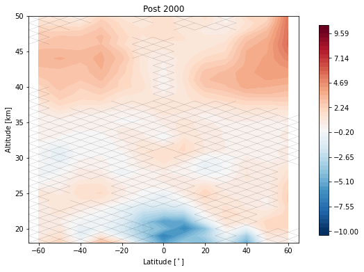
Now we remove the linear terms from our predictors and tell the regression call to post fit a trend to the residuals after the year 2000
[8]:
predictors = predictors.drop(['linear_pre', 'linear_post'], axis=1)

results = regress_all_bins(predictors, mzm_data['relative_anomaly'], tolerance=0.1, post_fit_trend_start='2000-01-01')

# Convert to ~ percent
results *= 100

trends.post_with_confidence(results, x='mean_latitude', y='altitude', ylim=(18, 50), log_y=False, figsize=(8, 6),
                                x_label='Latitude [$^\circ$]', y_label='Altitude [km]',
                                post_title='Post 2000')
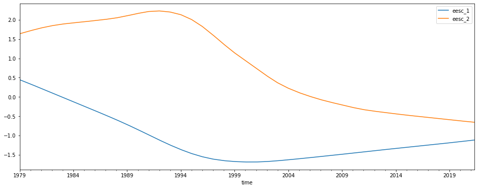
Lastly we add two orthogonal EESC terms and redo the regression
[9]:
predictors[['eesc_1', 'eesc_2']] = download.load_orthogonal_eesc('/media/users/data/LOTUS/proxies/EESC_Damadeo/eesc.txt')[['eesc_1', 'eesc_2']]

predictors[['eesc_1', 'eesc_2']].plot(figsize=(16, 6))

results = regress_all_bins(predictors, mzm_data['relative_anomaly'], tolerance=0.1)
The results are trickier to interpret, but we can combine the two EESC terms to find the total contribution in each bin for the EESC
[10]:
predictors = predictors[(predictors.index >= mzm_data.time.values[0]) & (predictors.index <= mzm_data.time.values[-1])]

eesc_contrib = results['eesc_1'].values[:, :, np.newaxis] * predictors['eesc_1'].values[np.newaxis, np.newaxis, :] +\
               results['eesc_2'].values[:, :, np.newaxis] * predictors['eesc_2'].values[np.newaxis, np.newaxis, :]

plt.plot(mzm_data.time.values, eesc_contrib[2, 40, :].T)
np.shape(eesc_contrib)
plt.title('EESC Contribution at 45 S, 40 km')
---------------------------------------------------------------------------
InvalidComparison                         Traceback (most recent call last)
/opt/conda/envs/doc_env/lib/python3.6/site-packages/pandas/core/arrays/datetimelike.py in wrapper(self, other)
    115         try:
--> 116             other = _validate_comparison_value(self, other)
    117         except InvalidComparison:

/opt/conda/envs/doc_env/lib/python3.6/site-packages/pandas/core/arrays/datetimelike.py in _validate_comparison_value(self, other)
     95         elif not is_list_like(other):
---> 96             raise InvalidComparison(other)
     97

InvalidComparison: 1984-10-01T00:00:00.000000000

During handling of the above exception, another exception occurred:

TypeError                                 Traceback (most recent call last)
<ipython-input-1-6e9d2c370b51> in <module>
----> 1 predictors = predictors[(predictors.index >= mzm_data.time.values[0]) & (predictors.index <= mzm_data.time.values[-1])]
      2
      3 eesc_contrib = results['eesc_1'].values[:, :, np.newaxis] * predictors['eesc_1'].values[np.newaxis, np.newaxis, :] +\
      4                results['eesc_2'].values[:, :, np.newaxis] * predictors['eesc_2'].values[np.newaxis, np.newaxis, :]
      5

/opt/conda/envs/doc_env/lib/python3.6/site-packages/pandas/core/indexes/extension.py in wrapper(self, other)
    127
    128         op = getattr(self._data, opname)
--> 129         return op(other)
    130
    131     wrapper.__name__ = opname

/opt/conda/envs/doc_env/lib/python3.6/site-packages/pandas/core/ops/common.py in new_method(self, other)
     63         other = item_from_zerodim(other)
     64
---> 65         return method(self, other)
     66
     67     return new_method

/opt/conda/envs/doc_env/lib/python3.6/site-packages/pandas/core/arrays/datetimelike.py in wrapper(self, other)
    116             other = _validate_comparison_value(self, other)
    117         except InvalidComparison:
--> 118             return invalid_comparison(self, other, op)
    119
    120         dtype = getattr(other, "dtype", None)

/opt/conda/envs/doc_env/lib/python3.6/site-packages/pandas/core/ops/invalid.py in invalid_comparison(left, right, op)
     32     else:
     33         typ = type(right).__name__
---> 34         raise TypeError(f"Invalid comparison between dtype={left.dtype} and {typ}")
     35     return res_values
     36

TypeError: Invalid comparison between dtype=period[M] and datetime64
With some annoying time conversions we can also find the predicted turnaround time in each bin
[11]:
turnaround_index = np.argmin(eesc_contrib, axis=2)

turnaround_times = mzm_data.time.values[turnaround_index]

def to_year_fraction(date):
    def since_epoch(date): # returns seconds since epoch
        return time.mktime(date.timetuple())

    try:
        ts = (np.datetime64(date, 'ns') - np.datetime64('1970-01-01T00:00:00Z')) / np.timedelta64(1, 's')
    except:
        print(np.datetime64(date))
        return np.nan

    dt = datetime.utcfromtimestamp(ts)
    s = since_epoch

    year = dt.year
    startOfThisYear = datetime(year=year, month=1, day=1)
    startOfNextYear = datetime(year=year+1, month=1, day=1)

    yearElapsed = s(dt) - s(startOfThisYear)
    yearDuration = s(startOfNextYear) - s(startOfThisYear)
    fraction = yearElapsed / yearDuration

    return dt.year + fraction

turnaround_times = np.frompyfunc(to_year_fraction, 1, 1)(turnaround_times).astype(float)

turnaround_times[turnaround_index == 0] = np.nan
turnaround_times[turnaround_index == len(mzm_data.time.values)-1] = np.nan

plt.pcolor(mzm_data.mean_latitude.values, mzm_data.altitude.values, np.ma.masked_invalid(turnaround_times.T))
plt.clim(1984, 2010)
plt.ylim(20, 50)
plt.ylabel('Altitude [km]')
plt.xlabel('Latitude')
plt.title('Turnaround Time')
plt.colorbar()
---------------------------------------------------------------------------
NameError                                 Traceback (most recent call last)
<ipython-input-1-c20e5a8ea2ea> in <module>
----> 1 turnaround_index = np.argmin(eesc_contrib, axis=2)
      2
      3 turnaround_times = mzm_data.time.values[turnaround_index]
      4
      5 def to_year_fraction(date):

NameError: name 'eesc_contrib' is not defined