Engine
Module: sasktran.engine
Engines are objects that can calculate radiances. Some of these engines can also calculate analytic or optimized Weighting Functions. One of the primary design objectives of SASKTRAN is to build a flexible radiative transfer framework so that the different components of a radiative transfer calculation are as modular as possible. This is our motivation for calling these objects engines as opposed to radiative transfer algorithms.
SASKTRAN’s primary engine product is SASKTRAN HR.
Base Class
Engines require a Geometry object, and an Atmosphere object at a minimum to get the gemetric and atmospheric specifications for the calculation.
- class sasktran.Engine(name: str, geometry: Geometry = None, atmosphere: Atmosphere = None, wavelengths: list = None, options: dict = None)
Bases:
objectBase class for objects which can perform radative transfer calculations.
- property atmosphere
The engines atmosphere definition object.
- Type:
- calculate_radiance(output_format='numpy', full_stokes_vector=False, stokes_orientation='geographic')
Calculate radiances.
- Parameters:
output_format (str, optional) – Determines the output format, one of [‘numpy’ or ‘xarray’]. If output_format=’numpy’, the radiance and optionally the weighting functions are returned as numpy arrays. If output_format=’xarray’ the radiance and weighting functions are returned inside of an xarray Dataset object.
full_stokes_vector (bool, optional) – If True, the full stokes vector is output. If False only the first element of the stokes vector is included. Note that setting this does not automatically enable vector calculations within the model, it only changes the output format, every model requires a different setting to be changed to change the calculation mode. Default: False
stokes_orientation (str, optional) – One of ‘geographic. The geographic basis is defined relative to the plane formed by the observer position and look vector. Here, Q, would be the linear polarization component for the nominal ‘up’ direction of an instrument. Default: ‘geographic’.
- Returns:
If output_format=’numpy’: The first np.ndarray is always the computed radiances. The shape of the computed radiances is (W, L) where W is the number of wavelengths, and L is the number of lines of sight. If
atmosphere.wf_species != Nonethen a second np.ndarray will be returned containing the computed weighting functions. The shape of this np.ndarray is engine specific but typically (W, L, A) where A is the number of altitudes at which at which the weighting functions were calculated. If full_stokes_vector is set to True, then what is returned is an array of sasktran.StokesVector objects.If output_format=’xarray’: A dataset containing the radiance and weighting functions with appropriate coordinates.
- Return type:
np.ndarray or np.ndarray, np.ndarray or xarray.Dataset
- property geometry
The engines geometry definition object.
- Type:
- property options
Dictionary map of additional engine options.
Examples
>>> import sasktran as sk
>>> engine = sk.EngineHR()
>>> engine.options['numordersofscatter'] = 1
- Type:
dict
- property wavelengths
Wavelengths in nm to perform the radiative transfer calculation at.
Examples
>>> import sasktran as sk
>>> engine = sk.EngineHR()
>>> engine.wavelengths = 600 # Single wavelength
>>> engine.wavelengths = [600, 340] # Multiple wavelengths
- Type:
np.ndarray or float
Note
Most engines have a lot of features and configuration options. We have tried to make engine
default configurations as reasonable as possible but obviously these defaults cannot efficiently
handle every possible case. Because of this, users have to be aware additional engine
configuration might be necessary to obtain efficinent and accurate results. These additional
configuration options are set through engine options (see sasktran.Engine.options).
SASKTRAN HR
SASKTRAN HR is our primary engine product. The HR engine solves the radiative transfer equation in a region of interest using the successive orders technique on a true spherical Earth. The main highlights of the engine are:
Support to calculate the Weighting Functions of target species
Adapative integration within optically thick regions
Polarized or scalar radiance calculations
Support for gradients across a region of interest using high resolution diffusive fields
Support for terminator conditions
Support for thermal emissions
Support for elevated surface topology
- class sasktran.EngineHR(geometry: Geometry | None = None, atmosphere: Atmosphere | None = None, wavelengths: list | None = None, options: dict | None = None)
Bases:
EngineExamples
>>> import sasktran as sk
>>> # configure your geometry
>>> geometry = sk.VerticalImage()
>>> geometry.from_sza_saa(60, 60, 0, 0, [10, 20, 30, 40], 54372, 0)
>>> # configure your atmosphere
>>> atmosphere = sk.Atmosphere()
>>> atmosphere['rayleigh'] = sk.Species(sk.Rayleigh(), sk.MSIS90())
>>> atmosphere.atmospheric_state = sk.MSIS90()
>>> atmosphere['o3'] = sk.Species(sk.O3DBM(), sk.Labow())
>>> atmosphere['no2'] = sk.Species(sk.NO2Vandaele1998(), sk.Pratmo())
>>> atmosphere.brdf = sk.Lambertian(0.3)
>>> # make your engine
>>> engine = sk.EngineHR(geometry=geometry, atmosphere=atmosphere, wavelengths=[350, 400, 450])
>>> rad = engine.calculate_radiance()
>>> print(rad)
[[ 0.11674...  0.10872...  0.04904...  0.01456...]
 [ 0.10837...  0.08537...  0.02897...  0.00804...]
 [ 0.10318...  0.06396...  0.01829...  0.00483...]]
- property atmosphere_dimensions
Sets the number of dimensions for the atmosphere in the radiative transfer calculation.
Input
Setting
1
One-dimensional in altitude
2
Two-dimensional in altitude and angle along the line of sight
3
Fully three-dimensional
Default: 1
- calculate_radiance(output_format='numpy', full_stokes_vector=False, stokes_orientation='geographic')
Calculate radiances.
- Parameters:
output_format (str, optional) – Determines the output format, one of [‘numpy’ or ‘xarray’]. If output_format=’numpy’, the radiance and optionally the weighting functions are returned as numpy arrays. If output_format=’xarray’ the radiance and weighting functions are returned inside of an xarray Dataset object.
full_stokes_vector (bool, optional) – If True, the full stokes vector is output. If False only the first element of the stokes vector is included. Note that setting this does not automatically enable vector calculations within the model, it only changes the output format, every model requires a different setting to be changed to change the calculation mode. Default: False
stokes_orientation (str, optional) – One of ‘geographic. The geographic basis is defined relative to the plane formed by the observer position and look vector. Here, Q, would be the linear polarization component for the nominal ‘up’ direction of an instrument. Default: ‘geographic’.
- Returns:
If output_format=’numpy’: The first np.ndarray is always the computed radiances. The shape of the computed radiances is (W, L) where W is the number of wavelengths, and L is the number of lines of sight. If
atmosphere.wf_species != Nonethen a second np.ndarray will be returned containing the computed weighting functions. The shape of this np.ndarray is engine specific but typically (W, L, A) where A is the number of altitudes at which at which the weighting functions were calculated. If full_stokes_vector is set to True, then what is returned is an array of sasktran.StokesVector objects.If output_format=’xarray’: A dataset containing the radiance and weighting functions with appropriate coordinates.
- Return type:
np.ndarray or np.ndarray, np.ndarray or xarray.Dataset
- cell_optical_depths()
Calculates the optical depths along each line of sight at each wavelength to each cell.
- Returns:
A two-dimensional list of shape (num_wavelength, num_los) where each element is a dictionary containing the keys ‘cell_start_optical_depth’ which has the optical depth at the start of the cell and ‘cell_start_distance’ which has the distance from the observer to the start of the cell along the line of sight vector.
- Return type:
List[List[Dict]]
- configure_for_cloud(grid_spacing_m: float, cloud_altitudes: array, cloud_diffuse_spacing_m: float = 100, max_optical_depth_of_cell: float = 0.01, min_extinction_ratio_of_cell: float = 1, max_adaptive_optical_depth: float = 2)
Configures the HR model for use with a cloud.
- Parameters:
grid_spacing_m (float) – Desired grid spacing of the model for all parameters exluding the cloud.
cloud_altitudes (np.array) – Altitudes that the cloud is non-zero at. [m]
cloud_diffuse_spacing_m (float, Optional) – Spacing in m that diffuse points should be placed inside the cloud. Lower values will result in a more accurate multiple scattering calculatino within the cloud. Default: 100 m
max_optical_depth_of_cell (float, Optional) – Maximumum optical depth that is allowed for the adaptive integration step within HR. Lower values will result in a more accurate calculation. Default: 0.01
min_extinction_ratio_of_cell (float, Optional) – The minimum ratio of extinction that must be hit for the adaptive integration to split a cell in two, between 0 and 1. Higher values will result in a more accurate calculation. It is recommended to leave this at 1 unless you know what you are doing. Default: 1
max_adaptive_optical_depth (float, Optional) – The maximum optical depth along the ray where splitting where occur. Default: 2
- property disable_los_single_scattering
Experimental option. If set to true, then single scattering along the line of sight is not calculated. Note that single scatter from the ground is still included if the line of sight intersects the Earth. Default: False.
- property grid_spacing
Sets many options dealing with general grids and discretizations in the model. In general, if you are interested in things on the scale of 1000 m, then set this to 1000 m. For most applications setting this property is sufficient, however for advanced users it may be necessary to set some grids individually.
Default: 1000 m
- property include_emissions
Enables support for atmospheric emissions inside the model. If set to True, any
Emissionobjects that are included in theAtmospherewill be used in the radiative transfer calculation. Note that the default value is False, ignoring emissions.Default: False
- property num_diffuse_profiles
Advanced option that controls the number of diffuse profiles in the model. If worried about the accuracy of the multiple scatter signal, this should be the first option to try changing. A diffuse profile represents a (latitude, longitude) where the multiple scatter signal is calculated. The default value of 1 indicates that the multiple scatter signal is only calculated at the reference point, or the average tangent point. If you increase the value to 5, then there will be 5 locations along the line of sight where the full multiple scatter calculation is done. Outside of these areas the multiple scatter signal is interpolated. Odd numbers of diffuse profiles are preferred (but not necessary) since this facilitates one profile being placed at the tangent point.
To determine if this setting has an effect on your calculation it is recommended to first compare the results between 1, 5, and 11 diffuse profiles.
The amount of diffuse profiles to obtain an accurate depends heavily on a variety of things, but most heavily the solar zenith and solar scattering angles. When the sun is high in the sky (low solar zenith angle) 1–3 diffuse profiles is usually sufficient. However, when looking across the solar terminator (sza ~90, ssa < 90) it might be necessary to use upwards of 50 diffuse profiles to obtain a signal accurate to better than 0.5%. More information on the number of required diffuse profiles can be found in Zawada, D. J., Dueck, S. R., Rieger, L. A., Bourassa, A. E., Lloyd, N. D., and Degenstein, D. A.: High-resolution and Monte Carlo additions to the SASKTRAN radiative transfer model, Atmos. Meas. Tech., 8, 2609-2623, https://doi.org/10.5194/amt-8-2609-2015, 2015.
- property num_orders_of_scatter
Controls the number of orders of scatter used inside the model. The number of orders of scatter controls the accuracy of the model. When set to 1, only light directly scattered from the sun is accounted for, with no multiple scattering.
The model runs substantially faster when set to 1 scatter order, therefore a common use case is to do development/testing with this property set to 1. There is very little speed difference between 2 orders of scatter and 50 orders of scatter, so usually it is recommended to set this to either 1 or 50.
Default: 50
- property num_threads
Controls the number of threads to use when multithreading the radiative transfer calculation. The default value of 0 indicates that the number of threads used will be equal to the number of available logical cores on the target machine.
Setting this value to a lower number than the number of available cores can be useful when running a radiative transfer calculation in the background and the computer is too slow to multitask.
Default: 0
- property polarization
The polarization mode of the model. Can either be set to ‘scalar’ or ‘vector’.
Default: ‘scalar’
- property prefill_solartransmission_table
Experimental option. If set to true, then the solar table will be prefilled instead of filling dynamically. Default: False.
- property refraction
Determines whether or not refraction effects should be included in the radiative transfer calculation. If set to true, then refraction effects will be considered where the model supports it. Currently this is only available for the observer line of sight rays (solar rays and multiple scattering will not account for refraction).
Note that refraction support is experimental and may have some side effects. Currently known limitations are that the surface_elevation and top_of_atmosphere_altitudeproperty may not work properly with refraction enabled.
Enabling refraction also changes the ray tracer slightly, meaning that calculations with and without refraction enabled may differ slightly due to integration accuracies/quadrature points, etc. It is recommended to experiment with the grid_spacing property to ensure that the calculation is done with enough precision.
Default: false
- property surface_elevation
Sets the elevation of the surface in [m] for the model. This setting can be used to account for changes in the Earth’s topography.
Default: 0 m
- property top_of_atmosphere_altitude
Sets the altitude of the top of the atmosphere. Above this altitude it is assumed there is no atmosphere. The default value of 100000 m is typically suitable for stratospheric applications but for the mesosphere it is sometimes necessary to increase this value.
Default: 100000 m
- property use_solartable_for_singlescatter
Experimental option. If set to true, then the solar table will be used for single scattering calculations instead of directly tracing solar rays. Default: False.
- class sasktran.EngineHRSSApprox(geometry: Geometry | None = None, atmosphere: Atmosphere | None = None, wavelengths: list | None = None, options: dict | None = None, ms_wavelengths: array | None = None)
Bases:
EngineHR- calculate_radiance(output_format='numpy', full_stokes_vector=False, stokes_orientation='geographic')
Calculate radiances.
- Parameters:
output_format (str, optional) – Determines the output format, one of [‘numpy’ or ‘xarray’]. If output_format=’numpy’, the radiance and optionally the weighting functions are returned as numpy arrays. If output_format=’xarray’ the radiance and weighting functions are returned inside of an xarray Dataset object.
full_stokes_vector (bool, optional) – If True, the full stokes vector is output. If False only the first element of the stokes vector is included. Note that setting this does not automatically enable vector calculations within the model, it only changes the output format, every model requires a different setting to be changed to change the calculation mode. Default: False
stokes_orientation (str, optional) – One of ‘geographic. The geographic basis is defined relative to the plane formed by the observer position and look vector. Here, Q, would be the linear polarization component for the nominal ‘up’ direction of an instrument. Default: ‘geographic’.
- Returns:
If output_format=’numpy’: The first np.ndarray is always the computed radiances. The shape of the computed radiances is (W, L) where W is the number of wavelengths, and L is the number of lines of sight. If
atmosphere.wf_species != Nonethen a second np.ndarray will be returned containing the computed weighting functions. The shape of this np.ndarray is engine specific but typically (W, L, A) where A is the number of altitudes at which at which the weighting functions were calculated. If full_stokes_vector is set to True, then what is returned is an array of sasktran.StokesVector objects.If output_format=’xarray’: A dataset containing the radiance and weighting functions with appropriate coordinates.
- Return type:
np.ndarray or np.ndarray, np.ndarray or xarray.Dataset
- Additional Documentation
For additional documentation and options see: https://arg.usask.ca/docs/SasktranIF/hr.html.
SASKTRAN-DO
SASKTRAN-DO is a radiative transfer engine similar to the well known DISORT and (V)LIDORT radiative transfer algorithms.
- class sasktran.EngineDO(geometry: Geometry | None = None, atmosphere: Atmosphere | None = None, wavelengths: list | None = None, options: dict | None = None)
Bases:
EngineExamples
>>> import sasktran as sk
>>> # Configure the geometry
>>> geometry = sk.NadirGeometry()
>>> tempo = sk.Geodetic()
>>> tempo.from_lat_lon_alt(0, -100, 35786000)
>>> lats = np.linspace(20, 50, 4)
>>> lons = np.linspace(-110, -90, 3)
>>> lats, lons = np.meshgrid(lats, lons, indexing='ij')
>>> geometry.from_lat_lon(mjd=57906.63472, observer=tempo, lats=lats, lons=lons)
>>> # Configure the atmosphere
>>> atmosphere = sk.ConstituentAtmosphere()
>>> atmosphere['rayleigh'] = sk.Species(sk.Rayleigh(), sk.MSIS90())
>>> atmosphere['o3'] = sk.Species(sk.O3DBM(), sk.Labow())
>>> atmosphere['no2'] = sk.Species(sk.NO2Vandaele1998(), sk.Pratmo())
>>> atmosphere.brdf = sk.Kokhanovsky()
>>> # Calcualte radiance
>>> engine = sk.EngineDO(geometry=geometry, atmosphere=atmosphere, wavelengths=[350, 450])
>>> rad = engine.calculate_radiance('numpy')
>>>
>>> # print radiances
>>> print(rad[0].reshape((4, 3))) # radiance at 350nm
[[ 0.15726175  0.19468353  0.22767423]
 [ 0.1666762   0.20027906  0.22962238]
 [ 0.17116222  0.1995542   0.22411801]
 [ 0.17099479  0.1932349   0.21235274]]
>>> print(rad[1].reshape((4, 3))) # radiance at 450nm
[[ 0.15884236  0.19815234  0.23287579]
 [ 0.16822132  0.20341264  0.23415734]
 [ 0.17226753  0.20184478  0.22736965]
 [ 0.1716201   0.19441591  0.21402527]]
- property alt_grid
Internal altitude grid inside the model. ALl climatologies/optical properties are sampled on this grid, and then integrated over it to find the layer quantities. Default: Linearly spaced from 0 to 100 km with spacing of 0.5 km
- calculate_radiance(output_format='xarray')
Calculate radiances.
- Parameters:
output_format (str, optional) – Determines the output format, one of [‘numpy’ or ‘xarray’]. If output_format=’numpy’, the radiance and optionally the weighting functions are returned as numpy arrays. If output_format=’xarray’ the radiance and weighting functions are returned inside of an xarray Dataset object.
full_stokes_vector (bool, optional) – If True, the full stokes vector is output. If False only the first element of the stokes vector is included. Note that setting this does not automatically enable vector calculations within the model, it only changes the output format, every model requires a different setting to be changed to change the calculation mode. Default: False
stokes_orientation (str, optional) – One of ‘geographic. The geographic basis is defined relative to the plane formed by the observer position and look vector. Here, Q, would be the linear polarization component for the nominal ‘up’ direction of an instrument. Default: ‘geographic’.
- Returns:
If output_format=’numpy’: The first np.ndarray is always the computed radiances. The shape of the computed radiances is (W, L) where W is the number of wavelengths, and L is the number of lines of sight. If
atmosphere.wf_species != Nonethen a second np.ndarray will be returned containing the computed weighting functions. The shape of this np.ndarray is engine specific but typically (W, L, A) where A is the number of altitudes at which at which the weighting functions were calculated. If full_stokes_vector is set to True, then what is returned is an array of sasktran.StokesVector objects.If output_format=’xarray’: A dataset containing the radiance and weighting functions with appropriate coordinates.
- Return type:
np.ndarray or np.ndarray, np.ndarray or xarray.Dataset
- property layer_construction
Method used to place the layer boundaries in altitude. Should be one of uniform_pressure for uniform pressure layers, uniform_optical_depth for layers of equal optical depth, uniform_height for layers spaced linearly in height, match_altitude_grid to match layers with the internal altitude grid, or a numpy array of altitudes for manually specified layer boundaries. Default: uniform_pressure
- property num_brdf_quadrature_terms
The number of quadrature terms used to calculate the Legendre coefficients for the BRDF. Only has an effect if a Non-Lambertian surface is being used. Default: 64
- property num_spherical_sza
Number of solar zenith angles to calculate the plane parallel solution at when operating in spherical mode. Default: 2
- property num_stokes
Number of stokes parameters to include in the calculation and output. Set to 1 for scalar calculations, and to 3 for vector calculations. Default: 1
- property num_streams
The number of streams used inside the calculation. Together with the number of layers, the number of streams is one of the primary settings that controls the accuracy of the model. Default: 16
- property num_threads
Number of threads to use in the calculation when running on multiple wavelengths. The value of 0 indicates use every logical core present on the machine. It is recommended to set this value to the number of physical cores on the machine for maximum performance. Default: 0
- property viewing_mode
Geometry viewing mode of the model for the line of sight rays, either spherical or plane_parallel. Default: plane_parallel
SASKTRAN-TIR
SASKTRAN-TIR is a spherical radiative transfer engine designed for the thermal infrared regime where scattering is negligible.
- class sasktran.EngineTIR(geometry: Geometry | None = None, atmosphere: Atmosphere | None = None, wavelengths: list | None = None, options: dict | None = None)
Bases:
EngineExamples
>>> import sasktran as sk
>>> import numpy as np
>>> from sasktran.tir.engine import EngineTIR
>>> from sasktran.tir.opticalproperty import HITRANChemicalTIR
>>> # Select wavenumbers to do calculation at
>>> wavenum = np.linspace(775.0, 775.003, 4)
>>> # Wavelengths passed to engine must in increasing order
>>> wavelen = 1.0e7 / wavenum[::-1]
>>> # Create limb view geometry for a 20 km tangent altitude observed from a 40 km balloon altitude
>>> geometry = sk.VerticalImage()
>>> geometry.from_sza_saa(60, 60, 0, 0, [10, 20, 30, 40], 54372, 0)
>>> # Create an atmosphere with absorbing/emitting ozone
>>> atmosphere = sk.Atmosphere()
>>> o3_opt = HITRANChemicalTIR('O3', micro_window_margin=50)
>>> atmosphere['ozone'] = sk.Species(o3_opt, sk.Labow())
>>> # Create the engine and perform the calculation
>>> engine = EngineTIR(geometry=geometry, atmosphere=atmosphere, wavelengths=wavelen)
>>> rad = engine.calculate_radiance()
>>> print(rad)
[[8.73341577e+12 1.09506519e+13 1.32697534e+13 4.41957608e+12]
 [1.47059359e+13 1.67048571e+13 2.02328109e+13 1.51375632e+13]
 [1.06787128e+13 1.28978370e+13 1.59440769e+13 7.41160317e+12]
 [5.22908338e+12 7.13817250e+12 7.17447283e+12 9.33290088e+11]]
- property adaptive_integration
A boolean property that, if True, enables dynamic cell splitting during the radiative transfer integration. During the ray tracing process, the line of sight is split into cells based on the intersection of the line of sight with geometric shapes used to split the atmosphere into homogeneous layers. When the optical depth of a cell is computed, the cell is split if one or both of the following conditions are satisfied:
The optical depth of the cell exceeds the value specified by the property
max_optical_depth_of_cellThe ratio of the smaller of the two values of extinction at the endpoints of the cell to the larger value is less than the property
min_extinction_ratio_of_cell
Default: True
- property atmosphere_dimensions
Sets the number of dimensions for the atmosphere in the radiative transfer calculation.
Input
Setting
1
One-dimensional in altitude
2
Two-dimensional in altitude and along along the line of sight
Default: 1
- calculate_radiance(output_format='numpy', full_stokes_vector=False)
Calculate radiances.
- Parameters:
output_format (str, optional) – Determines the output format, one of [‘numpy’ or ‘xarray’]. If output_format=’numpy’, the radiance and optionally the weighting functions are returned as numpy arrays. If output_format=’xarray’ the radiance and weighting functions are returned inside of an xarray Dataset object.
full_stokes_vector (bool, optional) – If True, the full stokes vector is output. If False only the first element of the stokes vector is included. Note that setting this does not automatically enable vector calculations within the model, it only changes the output format, every model requires a different setting to be changed to change the calculation mode. Default: False
stokes_orientation (str, optional) – One of ‘geographic. The geographic basis is defined relative to the plane formed by the observer position and look vector. Here, Q, would be the linear polarization component for the nominal ‘up’ direction of an instrument. Default: ‘geographic’.
- Returns:
If output_format=’numpy’: The first np.ndarray is always the computed radiances. The shape of the computed radiances is (W, L) where W is the number of wavelengths, and L is the number of lines of sight. If
atmosphere.wf_species != Nonethen a second np.ndarray will be returned containing the computed weighting functions. The shape of this np.ndarray is engine specific but typically (W, L, A) where A is the number of altitudes at which at which the weighting functions were calculated. If full_stokes_vector is set to True, then what is returned is an array of sasktran.StokesVector objects.If output_format=’xarray’: A dataset containing the radiance and weighting functions with appropriate coordinates.
- Return type:
np.ndarray or np.ndarray, np.ndarray or xarray.Dataset
- property do_temperature_wf
Set this property to True to enable temperature weighting function calculations.
Default: False
- property do_vmr_wf
Controls the units of gas species weighting functions. The default setting configures weighting functions to be given in (radiance / number density) where number density has units of cm^-3. Setting this property to True tells the engine to calculate weighting functions with units of (radiance / VMR).
Default: False
- property grid_spacing
Sets the vertical spacing of homogeneous atmosphere layers in [m].
Default: 1000 m
- property ground_emissivity
Sets the scalar emissivity of the surface of the Earth. If the line of sight ends at the ground, the emission from the Earth’s surface must be taken into account. In the TIR engine this emission is modelled as a black body with constant emissivity. For limb-viewing geometries this setting will have no effect as there are no scattering effects in the TIR engine.
Default: 1
- property linear_extinction
If this property is set to True, the engine calculates the optical depth of a cell by allowing the extinction to vary linearly with height, between the values at the endpoints of the cell. If this property is set to False, the extinction of a cell is constant, calculated as the average of the values at the endpoints.
Default: True
- property max_optical_depth_of_cell
Set the maximum optical depth of a single cell is allowed to have before it is split into two cells, when adaptive integration is enabled. If the property
adaptive_integrationis set to False, this property has no effect.Default: 0.1
- property min_extinction_ratio_of_cell
Set the minimum ratio between the extinction at the endpoints of single cell that is allowed before the cell is split, when adaptive integration is enabled. If the property
adaptive_integrationis set to False, this property has no effect. The ratio is calculated as the smaller of the two extinction values divided by the larger.Default 0.9
- property num_threads
Controls the number of threads to use when multithreading the radiative transfer calculation. The default value of 0 indicates that the number of threads used will be equal to the number of available logical cores on the target machine.
Setting this value to a lower number than the number of available cores can be useful when running a radiative transfer calculation in the background and the computer is too slow to multitask.
Default: 0
- property refraction
If set to true, then refractive ray tracing is performed for the observer line of sight rays.
Default: false
- property surface_elevation
Sets the surface elevation in meters.
Default: 0 m
- property top_of_atmosphere_altitude
Sets the altitude of the top of the atmosphere. Above this altitude it is assumed there is no atmosphere. Due to the assumption of local thermodynamic equilibrium within the Thermal InfraRed engine, increasing the value above 100000 m is not recommended because this simplification can not be used at higher altitudes.
Default: 100000 m
- property use_cached_cross_sections
Designed to enable faster iterative radiance calculations, this setting instructs the TIR engine to compute cross sections using cached results. This can only be done if:
calculate_radiance()has been called at least onceThe only change to the engine object since the last call to
calculate_radiance()is the number density climatology of one or more species in the atmosphere property. The optical properties used for these species must the same; if a new optical property is specified, the resulting radiance will be as though the old optical property were used.The species whose climatologies have been changed must also be set as the
wf_speciesof the atmosphere property, i.e. only the species for which weighting functions are computed may have their climatologies changed
Default: True
- property wavelengths
Wavelengths in nm to perform the radiative transfer calculation at.
Examples
>>> import sasktran as sk
>>> engine = sk.EngineHR()
>>> engine.wavelengths = 600 # Single wavelength
>>> engine.wavelengths = [600, 340] # Multiple wavelengths
- Type:
np.ndarray or float
- property wf_heights
Heights, in meters, to compute analytic weighting functions at.
Default:
np.linspace(500, 99500, 100)# 500, 1500, 2500, …, 99500
- property wf_widths
Weighting function widths. The weighting functions determine the effect of perturbing a species population at each height specified by
wf_heightson the radiance. The property wf_widths species the vertical distance from each value inwf_heightsto the height where the perturbation is zero. Therefore,wf_heightsandwf_widthsmust have identical lengths.i.e. for a weighting function calculation at
wf_heights[i], the perturbation is maximum atwf_heights[i]and decreases linearly (with height) to 0 at(wf_heights[i] - wf_widths[i])and(wf_heights[i] + wf_widths[i]).Default:
np.array([1000] * 100)# sets a width of 1000 m at every height in wf_heights
SASKTRAN-OCC
An occultation engine. This engine calculates the optical depth along a curved line of sight in the atmosphere.
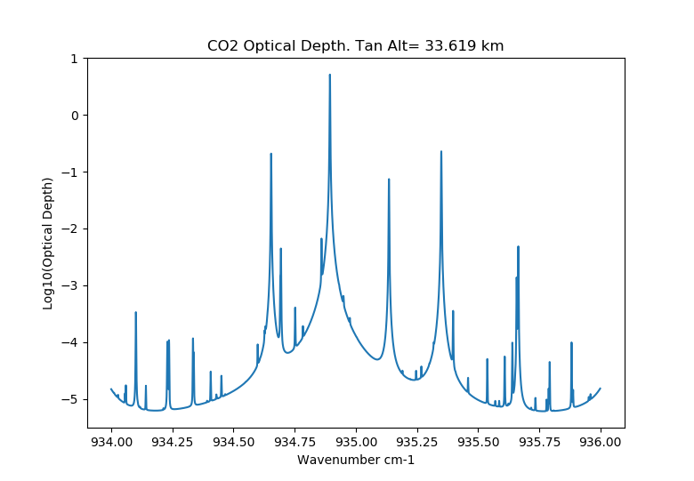
Figure generated from the data generated by the example given below.
- class sasktran.EngineOCC(geometry: Geometry | None = None, atmosphere: Atmosphere | None = None, wavelengths: List[float] | None = None, options: Dict[str, Any] | None = None)
Bases:
Engine” The
OCCengine was built as a radiative transfer model for solar occultation observations from a satellite. It was originally built as a plug-in subsititute engine for the Fortran code used in the ACE-FTS analysis and is well-suited for atmospheric transmission calculations in near infra-red and infra-red micro-windows. The algorithm traces curved rays using a spherically symmetric version of Snells law, Thompson et al. 1982. The refractive index of the atmosphere follows the dry-air formula published by Filippenko 1982 which only requires a single profile of pressure and temperature; we note that the atmospheric refractive index does not include effects due to moist air which may be significant at tropospheric altitudes.The code for the OCC engine was frequently compared to the original Fortran code during development to ensure they are identical. The engine calculates transmission through the atmosphere, rather than radiance, and has the following features:
curved ray tracing in a spherically symmetric atmosphere. The path length of the curved ray is the same as the ACE-FTS code to within 1 micron.
The code provides efficient calculation of Voigt profiles across micro-windows in the near infra-red and infra-red.
References
Dennis A. Thompson, Theodore J. Pepin, and Frances W. Simon. Ray tracing in a refracting spherically symmetric atmosphere. J. Opt. Soc. Am., 72(11):1498–1501, Nov 1982. URL: http://www.osapublishing.org/abstract.cfm?URI=josa-72-11-1498, doi:10.1364/JOSA.72.001498.
A. V. Filippenko. The importance of atmospheric differential refraction in spectrophotometry. Publications of the Astronomical Society of the Pacific , 94:715–721, August 1982. doi:10.1086/131052.
Example
Here is an example that calculates the optical depth at 5000 wavenumbers across a CO2 band at 934 to 936 cm-1. This example is almost the same as ACE-FTS scan ace.sr20314 except the sun is no longer in the correct location. The test example creates a user defined profile of CO2 number density used for CO2 absorption and the MSIS climatology for Rayleigh extinction. Lines of sights are specified as an array of tangent altitudes and the satellite is placed at 600 km. Optical depth through the atmosphere is calculated for each tangent altitude across the 4000 wavenumbers:
import numpy as np
import matplotlib.pyplot as plt
import sasktran as sk

def test_occ_engine():

    co2profile =  np.array( [    0.000, 9.5620350469e+15,  1000.000, 8.5604676285e+15,  2000.000, 7.7062120091e+15,  3000.000, 6.9531991470e+15,  4000.000, 6.2702731320e+15,  5000.000, 5.6375862919e+15,
                    6000.000, 5.0651291274e+15,  7000.000, 4.4975838604e+15,  8000.000, 3.9468136861e+15,  9000.000, 3.4348048814e+15, 10000.000, 2.9871067830e+15, 11000.000, 2.5656416175e+15,
                   12000.000, 2.1874053365e+15, 13000.000, 1.8533816021e+15, 14000.000, 1.6023327829e+15, 15000.000, 1.3568375796e+15, 16000.000, 1.1279532788e+15, 17000.000, 9.7672446573e+14,
                   18000.000, 8.4173283897e+14, 19000.000, 7.1576699275e+14, 20000.000, 6.2070908062e+14, 21000.000, 5.2364297410e+14, 22000.000, 4.3181248841e+14, 23000.000, 3.7860567983e+14,
                   24000.000, 3.2428122678e+14, 25000.000, 2.7110791383e+14, 26000.000, 2.3526785090e+14, 27000.000, 2.0344493146e+14, 28000.000, 1.7304110039e+14, 29000.000, 1.4714113133e+14,
                   30000.000, 1.2544180466e+14, 31000.000, 1.0738346125e+14, 32000.000, 9.2442937053e+13, 33000.000, 8.0342242281e+13, 34000.000, 6.9455591820e+13, 35000.000, 5.9095214441e+13,
                   36000.000, 5.0374561563e+13, 37000.000, 4.3515754800e+13, 38000.000, 3.7794009046e+13, 39000.000, 3.2874895083e+13, 40000.000, 2.8685628465e+13, 41000.000, 2.4978923024e+13,
                   42000.000, 2.1682117851e+13, 43000.000, 1.8864809592e+13, 44000.000, 1.6431826141e+13, 45000.000, 1.4348899126e+13, 46000.000, 1.2595260698e+13, 47000.000, 1.1093125765e+13,
                   48000.000, 9.8376261311e+12, 49000.000, 8.8026864921e+12, 50000.000, 7.8993464447e+12, 51000.000, 7.0038829664e+12, 52000.000, 6.0771348455e+12, 53000.000, 5.2887296427e+12,
                   54000.000, 4.6787494256e+12, 55000.000, 4.1667051367e+12, 56000.000, 3.6751620506e+12, 57000.000, 3.1811011797e+12, 58000.000, 2.7604364326e+12, 59000.000, 2.4249492298e+12,
                   60000.000, 2.1420175118e+12, 61000.000, 1.8772791073e+12, 62000.000, 1.6195294613e+12, 63000.000, 1.3994285676e+12, 64000.000, 1.2229247260e+12, 65000.000, 1.0734951007e+12,
                   66000.000, 9.3270881894e+11, 67000.000, 7.9345730980e+11, 68000.000, 6.7795327304e+11, 69000.000, 5.9174431127e+11, 70000.000, 5.2173619614e+11, 71000.000, 4.5523334147e+11,
                   72000.000, 3.8840635314e+11, 73000.000, 3.3304529951e+11, 74000.000, 2.9045416707e+11, 75000.000, 2.5517516779e+11, 76000.000, 2.2127024526e+11, 77000.000, 1.8582366434e+11,
                   78000.000, 1.5596546276e+11, 79000.000, 1.3362547386e+11, 80000.000, 1.1541990113e+11, 81000.000, 9.8756976417e+10, 82000.000, 8.2629944315e+10, 83000.000, 6.8563739750e+10,
                   84000.000, 5.6814363571e+10, 85000.000, 4.6797966799e+10, 86000.000, 3.8795906044e+10, 87000.000, 3.2908654369e+10, 88000.000, 2.7811184596e+10, 89000.000, 2.2974282383e+10,
                   90000.000, 1.8716304570e+10, 91000.000, 1.5254396937e+10, 92000.000, 1.2548308770e+10, 93000.000, 1.0295593615e+10, 94000.000, 8.3338827301e+09, 95000.000, 6.6488536883e+09,
                   96000.000, 5.2936443303e+09, 97000.000, 4.2242029799e+09, 98000.000, 3.3594428424e+09, 99000.000, 2.6511281727e+09]).reshape( [100,2])
    altitudes = co2profile[:,0]
    values    = co2profile[:,1]
    co2numberdensity = sk.ClimatologyUserDefined(altitudes, {'SKCLIMATOLOGY_CO2_CM3': values})

    atmosphere = sk.Atmosphere()
    atmosphere['rayleigh'] = sk.Species(sk.Rayleigh(), sk.MSIS90())
    atmosphere['co2']      = sk.Species(sk.HITRANChemical('CO2'), co2numberdensity )

    tanalts = np.array( [ 95.542934418655, 93.030998230911, 90.518486023880, 87.999366761185, 85.485855103470, 82.971916199661, 80.457603455521, 77.942962647415, 75.421955109573, 72.906806946732,
                 70.391479493118, 67.869934082962, 65.354396820999, 62.838825226761, 60.317182541824, 57.801700592972, 55.286336899734, 52.765050888992, 50.250070572830, 47.735359192825,
                 45.220966340042, 42.682148825007, 40.254586233282, 37.901745439957, 35.689252976524, 33.619203107470, 31.633878541417, 29.706157206720, 27.941217916525, 26.315136637345,
                 24.759740931714, 23.273057386890, 21.701357220703, 20.435203333687, 19.296175927224, 18.238125008002, 17.137857798933, 15.665431416870, 14.623809766528, 13.581115284387,
                 12.793781944543, 11.901170623281, 10.978181776555, 10.1851695349872, 9.4383271471788, 8.7424541473265, 8.0540969039894, 7.5483134223615, 7.0824804787830, 6.7903857771487,
                 6.3015475934096] )

    mjd = 54242.26386852                    # MJD("2007-05-22 06:19:58.24") Use ACE-FTS scan ace.sr20314 as an example.
    lat = 68.91
    lng = -79.65
    sza = 60.0
    saa = 157.5
    rayazi = 0.0
    geometry = sk.VerticalImage()
    geometry.from_sza_saa(sza, saa, lat, lng, tanalts, mjd, rayazi, satalt_km=600, refalt_km=20)

    wavenum = np.arange( 934.0, 936.0, 0.0005)
    wavelengths = 1.0E7/wavenum
    engine = sk.EngineOCC(geometry=geometry, atmosphere=atmosphere, wavelengths=wavelengths)

    extinction = engine.calculate_radiance()
    plt.plot( wavenum, np.log10(extinction[:,25]))
    plt.xlabel('Wavenumber cm-1')
    plt.ylabel('Log10(Optical Depth)')
    plt.title('CO2 Optical Depth. Tan Alt={:7.3f} km'.format(tanalts[25]))
    plt.show()
- property ray_tracing_wavenumber: float
Sets the wavenumber in cm-1 used for tracing curved rays through the atmosphere. Rays are only traced once in each model and the trajectories are shared between all wavenumber extinction calculations.
- Parameters:
wavenumber (float) – The wavenumber used for tracing rays.
- property userdefined_ground_altitude: float
Sets the altitude in meters of the ground shell above the oblate spheroid/sea level.
- Parameters:
heightm (float) – The height of the ground surface above sea-level in meters
- property userdefined_lines_of_sight_from_tangent_alt: ndarray
Adds a line of sight generated from the tangent height and an observer height.
- Parameters:
tangentheights (Array[2*n]) – A 2*n element array specifying
nlines of sight, the first element of each line of sight entry is the target tangent height and the 2nd element is the observer height. Both are in meters.
- property userdefined_lower_bound_altitude: float
The lower altitude of the atmosphere in meters used when considering the reference point
- Parameters:
heightm (float) – The minimum altitude in meters
- property userdefined_reference_point: ndarray
Sets the reference point to the given location.
- Parameters:
location (array[4]) – three element array specifing [latitude, longitude, height, mjd]. Note that the height field is ignored.
- property userdefined_reference_point_target_altitude: float
The target altitude to be used when determining the reference point. The target altitude is used in zenith and nadir observations to find the location where a ray intersects this altitude. This altitude is then used to find an average reference point location. The target altitude is used with the target range variable in limb viewing geometries to apply an increased weighting to lines of sight tangential in the vicinity of the target altitude. This encourages the reference point to be closer to the lines of sight which are tangential in the region of the reference point.
- Parameters:
heightm (float) – The target height in meters.
- property userdefined_reference_point_target_range: float
The reference point target range parameter. This variable is only used when calculating the reference point from limb viewing geometries. Specifies the altitude range above and below the target altitude for enhanced weighting of limb viewing lines of sight, default 15000 meters.
- Parameters:
range (float) – The height range value in meters.
- property userdefined_shells: ndarray
Configures the model to use the altitude shells defined by the user. The shell altitudes must be in ascending order and are specified in meters above sea level. By default, shell heights are evenly spaced at 1000 m intervals from 0 to 100,000 m. The diffuse points, by default, are placed in the middle of the shells and the optical properties are placed both in the middle and on the boundary of each shell.
- Parameters:
heights (array[n]) – The array of shell altitudes in meters above sea level.
- property userdefined_sun: ndarray
Manually sets the sun position. Use with caution as many line-of-sight helper functions will also set the sun’s position inside the internal engine.
- Parameters:
sun (array[3]) – The three element array of the sun’s unit vector. Expressed in global geographic coordinates and is in the directions from the Earth toward the sun.
- property userdefined_upper_bound_altitude: float
The maximum altitude of the atmosphere in meters used when considering the reference point
- Parameters:
heightm (float) – The maximum altitude in meters
SASKTRAN-MC
SASKTRAN MC is a fully spherical Monte Carlo radiative transfer engine, primarily used as a slow but accurate calibration for HR. It contains additional features as well, namely air mass factor calculation and rotational Raman scattering.
- class sasktran.EngineMC(geometry: Geometry | None = None, atmosphere: Atmosphere | None = None, wavelengths: list | None = None, options: dict | None = None)
Bases:
EngineExamples
>>> import sasktran as sk
>>> # configure your geometry
>>> geometry = sk.VerticalImage()
>>> geometry.from_sza_saa(60, 60, 0, 0, [10, 20, 30, 40], 54372, 0)
>>> # configure your atmosphere
>>> atmosphere = sk.Atmosphere()
>>> atmosphere['rayleigh'] = sk.Species(sk.Rayleigh(), sk.MSIS90())
>>> atmosphere.atmospheric_state = sk.MSIS90()
>>> atmosphere['o3'] = sk.Species(sk.O3DBM(), sk.Labow())
>>> atmosphere['no2'] = sk.Species(sk.NO2Vandaele1998(), sk.Pratmo())
>>> atmosphere.brdf = sk.Lambertian(0.3)
>>> # configure your options
>>> options = {'setmcdebugmode': 1234, 'setnumphotonsperlos': 500, 'setsolartabletype': 0}
>>> # make your engine
>>> engine = sk.EngineMC(geometry=geometry, atmosphere=atmosphere, wavelengths=[350, 400, 450], options=options)
>>> rad = engine.calculate_radiance()
>>> print(rad)
[[ 0.11689...  0.10768...  0.04666...  0.01477...]
 [ 0.10643...  0.08429...  0.02972...  0.00802...]
 [ 0.10589...  0.06424...  0.01797...  0.00499...]]
- property air_mass_factor
Sets the type of air mass factor calculation.
Input
Setting
0
No air mass factor calculation
1
Air mass factors calculated via path length
2
Air mass factors calculated via path optical depth
Default: 0
- property air_mass_factor_shells
Sets the altitudes that define the layers to calculate air mass factors in. Only relevant if air_mass_factor is not 0.
Default: 500 m intervals from 0 m to 100 000 m
- property air_mass_factor_species
Sets the species used for air mass factor optical depth calculations.
The first supported species listed by the climatology in the atmosphere object associated with this name will be used. If a supported species further down the list is required, set the ‘amfspecies’ option manually with a handle from sk.handles.standard_handles().
Only relevant if air_mass_factor is set to 2.
Default: None
- calculate_radiance(output_format='numpy', full_stokes_vector=False, stokes_orientation='geographic')
Calculate radiances.
- Parameters:
output_format (str, optional) – Determines the output format, one of [‘numpy’ or ‘xarray’]. If output_format=’numpy’, the radiance and optionally the weighting functions are returned as numpy arrays. If output_format=’xarray’ the radiance and weighting functions are returned inside of an xarray Dataset object.
full_stokes_vector (bool, optional) – If True, the full stokes vector is output. If False only the first element of the stokes vector is included. Note that setting this does not automatically enable vector calculations within the model, it only changes the output format, every model requires a different setting to be changed to change the calculation mode. Default: False
stokes_orientation (str, optional) – One of ‘geographic. The geographic basis is defined relative to the plane formed by the observer position and look vector. Here, Q, would be the linear polarization component for the nominal ‘up’ direction of an instrument. Default: ‘geographic’.
- Returns:
If output_format=’numpy’: The first np.ndarray is always the computed radiances. The shape of the computed radiances is (W, L) where W is the number of wavelengths, and L is the number of lines of sight. If
atmosphere.wf_species != Nonethen a second np.ndarray will be returned containing the computed weighting functions. The shape of this np.ndarray is engine specific but typically (W, L, A) where A is the number of altitudes at which at which the weighting functions were calculated. If full_stokes_vector is set to True, then what is returned is an array of sasktran.StokesVector objects.If output_format=’xarray’: A dataset containing the radiance and weighting functions with appropriate coordinates.
- Return type:
np.ndarray or np.ndarray, np.ndarray or xarray.Dataset
- property debug_mode
A non-zero value will fix the random number generator seed to that value and disable multi-threading.
Default: 0
- property max_optical_depth_of_cell
Set the maximum optical depth of a cell before the adaptive integrator will split it. Only relevant if optical_property_integration_type is 1.
Default: 0.1
- property max_photons_per_los
Sets the maximum number of photon paths to simulate for every line of sight. Simulation stops when this maximum or the target precision has been reached.
Default: 10000
- property max_raman_orders
Defines the maximum order of Raman scatter (equal to the length of the list), as well as the maximum total order of scatter for each order of Raman scatter (the first element corresponding to the first Raman order, and so on).
Setting this turns the optimized inelastic mode on; if it is left as an empty list, Raman scattering events will occur at the same rate they would physically. In optimized inelastic mode, Raman scattering events are forced in order to minimize the variance of the radiance, or the variance of the secondary output if secondary_output is not 0.
Only relevant if an inelastic species is included in the atmosphere.
Default: []
- property min_fraction_higher_order
Sets the fraction of samples that will automatically propagate to the highest order of scatter, regardless of contribution to the variance. Remaining samples will be truncated to minimize the variance with the minimum number of simulated scatter events. Set to 1.0 to disable this optimization.
Default: 0.1
- property min_fraction_higher_raman_order
Defines the fraction of all samples that will, for each order of Raman scatter, always be simulated up to the maximum total order defined by max_raman_orders. The length of min_fraction_higher_order must be one greater than the length of max_raman_order, with the extra element at the front of the list represent the 0th Raman order.
Another option is to specify a scalar here, which will be divided evenly among the Raman orders (this will likely not be optimal).
The purpose of these minimum fractions is to reduce the small bias introduced by using variance knowledge to determine what samples will be taken next.
Only relevant if an inelastic species is included in the atmosphere and max_raman_orders has length greater than 0.
Default: 0.1
- property min_relative_path_weight
MC simulation of a single photon path stops at some order if each higher-order scatter could add to the measured radiance by less than w*{amountAlreadyMeasured}. This can save a lot of time, as only the odd “important” high-order path has to be simulated, but it does introduce a small bias. The importance of each order of scattering decreases approximately geometrically (except if there are bright clouds, etc), so only the first truncated photon contributes significantly to this bias. A value of 0.0 indicates no truncation.
Choosing w = 1 / ( 3 * numPhotonsPerLOS^2 ) makes the negative bias approximately one third of the magnitude of random noise in the experiment. Very often a photon could make at most a contribution much less than w, so the bias is actually much smaller than might be expected.
Default: 0.0
- property num_optical_property_altitudes
Sets the number of evenly spaced altitudes for caching optical properties.
Default: 201
- property num_orders_of_scatter
Controls the number of orders of scatter used inside the model. The number of orders of scatter controls the accuracy of the model. When set to 1, only light directly scattered from the sun is accounted for, with no multiple scattering.
Default: 50
- property num_ray_tracing_shells
Sets the number of evenly spaced atmospheric shells used for ray tracing.
Default: 201
- property optical_property_integration_type
Set the optical property table integrator (quadrature) type. Adaptive will split the integration if the optical depth exceeds max_optical_depth_of_cell.
Input
Setting
0
Straight
1
Adaptive
Default: 0
- property optical_property_wavelengths
The wavelengths where optical properties will be cached. This is only relevant if inelastic radiance is being calculated. If inelastic scatters take a photon outside the range defined here, a warning will be thrown and optical properties will be extrapolated. If a single number is set here, it will be interpreted as a resolution and the wavelengths will be automatically set over a suitable range at this resolution.
Default: 1.0
- property optical_table_type
Sets the type of table used to hold the optical properties of the atmosphere.
Input
Setting
0
One-dimensional (altitude)
1
Three-dimensional (Delaunay sphere)
Default: 0
- property primary_wavelength
Sets the wavelength that will be used to guide the ray tracing when simultaneous_wavelength is True. If the wavelength set here does not belong to self.wavelengths, the nearest match will be used. If the wavelength set here is not positive, the wavelength nearest to the midpoint of the range will be used.
Default: -1.0
- property ray_tracer_type
Set the ray tracer type for rays from the sun into the atmosphere, rays for the observer line of sight, and rays traced during multiple scattering.
Solar rays should be straight – we don’t have a good algorithm for tracing curved rays from the sun to a point. MS rays should probably be straight – using curved rays has almost no effect and is a big performance hit. Using curved MS rays might be desireable for some people. LOS rays can be either straight or curved – the performance hit for curved rays is pretty small here.
Input
Setting
0
Straight ray tracing: straight rays intersecting spherical shells
1
Curved ray tracing: considering refraction
2
Generic ray tracing: straight rays intersecting arbitrary shapes
3
Curve the observer line of sight only
Default: 2
- property scatter_position_resolution
Sets the distance to determine the simulated scatter positions within.
Default: 50 m
- property secondary_output
Select secondary quantities to return alongside inelastic radiance. Only relevant if an inelastic species is included in the atmosphere.
Input
Setting
0
No secondary output
1
Elastic radiance
2
Ring spectrum
3
Filling-in parameter
Default: 0
- property simultaneous_wavelength
If true, multiple wavelengths will be calculated simultaneously using common ray tracing. This should not be used if air mass factors are being calculated.
Default: False
- property solar_irradiance
The solar spectrum used for inelastic radiance calculation, on the wavelength grid specified by optical_property_wavelengths. If a scalar is given, the solar spectrum will be constant.
Default: 1.0
- property solar_table_altitude_delta
Sets the altitude spacing for the solar transmission table. Only relevant if solar_table_type is 1 or 2.
Default: 500 m
- property solar_table_type
Sets the method for calculating solar transmissions.
Input
Setting
0
No table; solar transmissions calculated on the fly
1
Two-dimensional in altitude and solar zenith angle along the line of sight
2
Three-dimensional in altitude, solar zenith angle, and solar longitude
3
No solar contribution.
Default: 1
- property surface_elevation
Sets the elevation of the surface in [m] for the model. This setting can be used to account for changes in the Earth’s topography.
Default: 0 m
- property target_std
Sets the target for the relative precision of the simulation. Precision (stdev/result) varies as N^{-1/2}. Simulation stops when this target or the maximum number of photon paths has been reached.
Default: 0.01
- property top_of_atmosphere_altitude
Sets the altitude of the top of the atmosphere. Above this altitude it is assumed there is no atmosphere. The default value of 100000 m is typically suitable for stratospheric applications but for the mesosphere it is sometimes necessary to increase this value.
Default: 100000 m
See Also
- Geometry
Objects which describe the geometry of the calculations to the engine. At a minimum these objects define the Lines of Sight, but can also specify things such as the suns position and the polling reference point.
- Atmosphere
An object that describes the atmospheric constituents, and surface type to the engine. Atmospheric constituents are defined by a list of Species, and surfaces are defined by a given BRDF.