Basic Radiative Transfer Calculation with MC
In this example we perform a full radiative transfer calculation using the MC model. The example illustrates how the calculation can be truncated either by reaching a maximum number of samples or by reaching a target precision.
[1]:
%matplotlib inline
[2]:
import sasktran as sk
import matplotlib.pyplot as plt
import numpy as np
from sasktran.geometry import VerticalImage

tanalts_km = np.linspace(10, 50, 9)

# First recreate our geometry and atmosphere classes
geometry = VerticalImage()
geometry.from_sza_saa(sza=60, saa=60, lat=0, lon=0, tanalts_km=tanalts_km, mjd=54372, locallook=0,
                      satalt_km=600, refalt_km=20)

atmosphere = sk.Atmosphere()
atmosphere['ozone'] = sk.Species(sk.O3OSIRISRes(), sk.Labow())
atmosphere['air'] = sk.Species(sk.Rayleigh(), sk.MSIS90())
atmosphere.brdf = 1.0

# And now make the engine
engine = sk.EngineMC(geometry=geometry, atmosphere=atmosphere)

engine.max_photons_per_los = 300   # cap the calculation at 300 rays per line of sight
engine.target_std = 0.05           # stop if 5% precision is achieved
engine.solar_table_type = 0        # calculate single scatter source terms on the fly; no cache
engine.debug_mode = 1234           # disable multi-threading, fix rng seed for reproducibility

# Choose some wavelengths to do the calculation at
engine.wavelengths = [600, 340]

# And do the calculation
engine_output = engine.calculate_radiance()
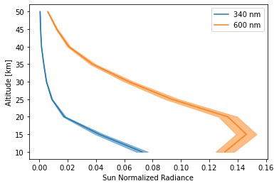
[3]:
rad = engine_output.radiance
stdev = np.sqrt(engine_output.radiance_variance)
for i in range(2):
    plt.plot(rad[i], tanalts_km, f'C{i}')
    plt.fill_betweenx(tanalts_km, rad[i] - stdev[i], rad[i] + stdev[i], color=f'C{i}', alpha=0.5)

plt.xlabel('Sun Normalized Radiance')
plt.ylabel('Altitude [km]')
plt.legend(['340 nm', '600 nm'])

plt.show()
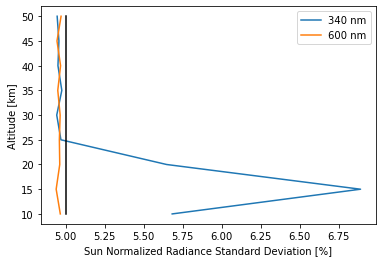
[4]:
rad = engine_output.radiance
stdev = np.sqrt(engine_output.radiance_variance)

# lower altitudes at 340 nm reached 300 samples before 5% precision
plt.plot(100 * stdev[0] / rad[0], tanalts_km, f'C{0}')
# all altitudes at 600 nm reached 5% precision before 300 samples
plt.plot(100 * stdev[1] / rad[1], tanalts_km, f'C{1}')

plt.plot([5, 5], [10, 50], 'k')
plt.xlabel('Sun Normalized Radiance Standard Deviation [%]')
plt.ylabel('Altitude [km]')
plt.legend(['340 nm', '600 nm'])

plt.show()