Concepts
skimpy is a python package that provides a framework to model the signals measured by optical instruments remotely sensing the Earth’s atmosphere at optical and infra-red wavelength. The package is useful for providing realistic inputs for instrument simulation studies and instrument design analysis.
The package sub-divides the problem into two separate parts. The first part calculates radiance incident upon the front-end optics of an instrument while the second stage propagates the signals from the front-end optics through the instrument to generate back-end signals.
Front-End Optics
The front-end optics of an instrument within the skimpy framework are described as an array of SpectralWindow
objects where each SpectralWindow combines a field-of-view with a wavelength definition. The field of view
defines an array of look vectors for the radiative transfer calculation and the wavelength definition defines the wavelengths
used in the radiative transfer calculation.
We show an example below where we create an instance of FrontEndOptics. We create two field of view objects
representing two rectangular, solid angle, areas that illuminate the front aperture of the optics. We create three wavelength
definition objects. Two of the objects use 30 wavelengths to cover the range of Gaussian spectral response function centered on 452 nm
with FWHM of 0.3 and 0.4 nm repsectively. The third wavelength definition implements a user defined spectral
response function, which is a triangular shape peaking at 457 nm and stepping from 454 nm to 460.0 in 0.1 nm steps.
Six different selections of the two fields of view and three wavelength definitions are combined to create six spectral windows which are added to the front-end optics object.:
def make_multifov_multiwave_instrument(self):

    front_end_optics = FrontEndOptics()

    fov0 = FOV_Rectangle(Hrange=(5, math.radians(0.0), math.radians(0.5)),                                          # Horizontal field of view is 5 points spanning 0.0 to 0.5 degrees in front_end_optics control frame
                         Vrange=(3, math.radians(0.0), math.radians(20.0 / 3600.0)))                                # Vertical field of view is 3 points spanning 0.0 to 20 arc seconds in front_end_optics control frame

    fov1 = FOV_Rectangle(Hrange=(5, math.radians(0.2), math.radians(0.5)),                                          # Horizontal field of view is 5 points 0.2 to 0.5 degrees in front_end_optics control frame
                         Vrange=(3, math.radians(0.0), math.radians(20.0 / 3600.0)))                                # Vertical field of view is 3 points spanning 0.0 to 20 arc seconds in front_end_optics control frame

    wav0 = WavelengthGaussianSRF(30, 450.0, 0.3)                                                                    # wavelength region 1. 30 wavelengths across 450 nanometers, FWHM = 0.53 nm
    wav1 = WavelengthGaussianSRF(30, 452.0, 0.4)                                                                    # The code will spectrally integrate over each wavelength region

    srf_wavelen = np.arange(454.0, 460.0, 0.1)                                                                      # define a set of wavelengths for a user defined SRF
    srf = 3.0 - np.abs(457.00 - srf_wavelen)                                                                        # create the user defined SRF. This is a triangular pyramid shape
    wav2 = WavelengthUserdefinedSRF(srf, srf_wavelen)                                                               # Create the user defined wavelength definition

    front_end_optics.add_spectral_window(SpectralWindow(front_end_optics, fov0, wav0))                              # define the spectral_windows used in the simulation
    front_end_optics.add_spectral_window(SpectralWindow(front_end_optics, fov0, wav1))                              # Each spectral_window is a combination of a wavelength range and a field of view
    front_end_optics.add_spectral_window(SpectralWindow(front_end_optics, fov0, wav2))                              # The front-end back_end_radiance will be integrated over the eavelength range and the field of view
    front_end_optics.add_spectral_window(SpectralWindow(front_end_optics, fov1, wav0))
    front_end_optics.add_spectral_window(SpectralWindow(front_end_optics, fov1, wav1))
    front_end_optics.add_spectral_window(SpectralWindow(front_end_optics, fov1, wav2))
    return front_end_optics
See also
Field of View
Fields of view are defined using instrument coordinates where \(\hat{x}_{icf}\) is the instrument boresight and \(\hat{y}_{icf}\) and \(\hat{z}_{icf}\) are the two orthogonal axes, usually parallel to the rows or columns of the detector.
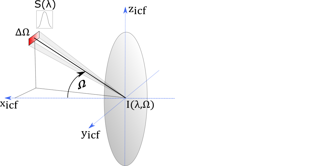
Fig. 1 Fields of view are defined in the instrument control frame.
The user should understand that the moniker of “field of view” only refers to an area of solid angle at the front aperture and does not have to correspond to the real field of view of any given instrument. For example, 2-D imager studies will often design field of view objects with small, front-end solid angles that map to small pixelated areas on the detector plane. Conversely, single slit spectrograph studies will often create a field of view object with a solid angle at the front-end that matches the instrument’s actual field of view.
The skimpy code has been designed to support a variety of field-of-view shapes but currently only has an implementation for rectangular shapes. Circular fields of view will be coming soon.
See also
Platforms
The instrument is mounted (in software) on a suitable Platform object either chosen from the skretrieval package or a custom platform derived form the Plaform base class. The Platform is positioned and orientated in space and time using various platform-specific techniques outlined in the skretrieval documentation. The Platform class, once positioned and rotated, generates rotation matrices to convert the fields of view defined in the instrument control frame to the ECEF position and look unit-vectors required by the radiative transfer models.
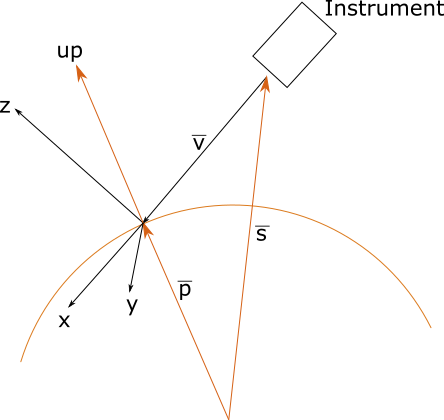
Fig. 2 Platforms convert fields of view into ECEF position and look vectors.
See also
More detail in the Platforms section of the skretrieval documentation.
Wavelength Definition
Wavelength definitions specify the range of wavelengths to be used in radiative transfer calculations. In the simplest option the user explicitly specifies the wavelengths at which they wish calculations. More sophisticated options allow the user to specify the choice of wavelengths using less direct methods, distributing points across a spectral response function for example.
The choices and options used to create the wavelength definitions are coupled with options given to the Front-End Radiance Generator used to calculate radiances. This combination of options, some from the wavelength definitions and others from the front-end radiance generator can be used to select optimizations that produce radiances at higher spectral resolution than those given in the wavelength definition.
UVIS-NIR: TOA Albedo to Radiance Methods
Radiative transfer models for the UVIS-NIR spectral regions, such as Sasktran HR, internally calculate the top-of-atmosphere albedo, which can be thought of as an effective atmospheric transmission. The radiance signal is quickly calculated from the product of the top-of-atmosphere albedo and the solar spectral irradiance, i.e.
where \(R(\lambda)\) is the radiance, \(S(\lambda)\) is the solar spectral irradiance and \(A(\lambda)\) is the top-of-atmosphere albedo. This equation is valid across the UVIS-NIR spectral region although we note it does not account for in-elastic scattering (Raman etc.) or photo-chemical emission terms, both of which are assumed to be negligible within these models.
Three configurations for converting the calculated toa albedo signal to radiance value are implemented in the UVIS-NIR,
Front-End Radiance Generator, FrontEndRadianceGeneratorHR. The three methods are listed in the table below.
UVIS-NIR Optimization Parameter |
Description |
|---|---|
Interpolate the calculated TOA Albedo to the solar spectrum sampling and then apply the solar spectrum |
|
Interpolate the solar spectrum to the wavelengths in the |
|
Convolve the high resolution solar spectrum with a Gaussian before applying to the calculated TOA albedo |
The user must explicitly choose which conversion method they wish to use when they calling the UVIS-NIR front end radiance generator and they must construct wavelength definitions to match the chosen method.
See also
interpolate_user_to_solar_wavelengths
This optimization allows the user to generate radiances on a high spectral sample grid using a few RTM calculation wavelengths. The toa albedo is calculated by the radiative transfer model on a coarse sampling grid and linearly interpolated to the sample spacing of the built-in solar spectral irradiance, typically 0.01 nm. It is useful when the user wishes to calculate radiance on a high resolution wavelength grid but knows, a-priori, that the toa-albedo can be accurately calculated and interpolated on a much coarser grid.
where \(L\) is a linear interpolation factor and \(A_{coarse}[i]\) is the array of coarse albedo values.
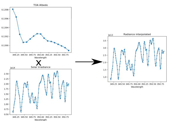
Fig. 3 High resolution radiances can be generated by interpolating low resolution TOA Albedo signals to the solar irradiance resolution.
This can be an important optimization technique for calculating signals across various visible spectral features such as ozone, nitrogen dioxide, aerosols and others.
Note
The radiance array is returned at the sampling spacing of the built in solar irradiance. The user must have a-priori knowledge of the spectral region they are modelling to ensure the toa interpolation is appropriate.
interpolate_solar_to_user_wavelengths
This option is useful for users who wish to calculate radiance at very high resolution with sample spacings shorter than the sampling of the built-in solar spectral irradiance, typically 0.01 nm. This scenario is often encountered when modelling Voigt profiles in the NIR.
In this technique the solar irradiance data are linearly interpolated to the toa albedo wavelength grid. The option does not offer any optimization as toa albedo is calculated by the radiative transfer model at every wavelength specified by the user.
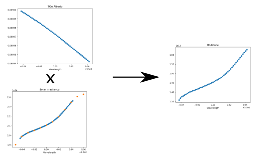
Fig. 4 Very high resolution radiances can be generated by interpolating solar irradiance to the toa albedo wavelengths.
preconvolved_solar
This option provides the ability to model incident radiance averaged across a spectral response function using an RTM calculation at only one wavelength and a preconvolved solar irradiance.
The technique is the fastest of the three options as it only requires calculation at one wavelength. But is also the
least accurate as it implicitly assumes the toa albedo is constant across the non-zero regions of the spectral response
function, see Background section below. The technique also demands that a spectral response function is specified with
the wavelength definition, this is enforced by demanding that this technique can only use classes derived from
WavelengthDefinitionSRF
The option radiances incident at the front end optics that include an instrumental spectral response function (SRF a.k.a. PSF) that is pre-convolved with the solar spectrum. This technique is appropriate when it is reasonable to assume the toa albedo signal is constant across the (non-zero) wavelength range of the instrument spectral response function.
It has the advantage that it only requires calculation of the toa albedo at one wavelength, typically the the central wavelength of the spectral response function.
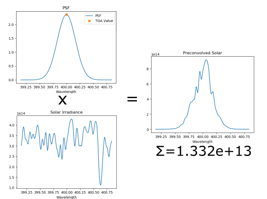
Fig. 5 High resolution convolution of instrument PSF with solar irradiance at one wavelength.
The preconvolved solar signal is generated by integrating the product of the solar spectrum and the instrument spectral response function. The radiance is estimated as the product of the toa albedo at the central wavelength and the preconvolved solar signal
Note
This mode will only return the radiance at one wavelength. The wavelength definition object must derive from class
WavelengthDefinitionPSF to provide the instrument spectral response function and other information to the
front end radiance generator.
Background
The convolution of the high resolution radiance signal and the instrument SRF is given by
where \(F(\lambda_0 - \lambda)\) is the spectral response function of the instrument and \(R_{conv}(\lambda_0)\) is the convolved radiance signal at wavelength , \(\lambda_0\). We can immediately substitute the formula for \(R(\lambda)\) to give,
If we make the approximation that the toa albedo signal, \(A(\lambda)\), has a constant value, \(A(\lambda_0)\), across the range of integration then,
or
where \(S_{conv}(\lambda_0)\) is the preconvolved solar spectrum given by,
Front-End Radiance Generator
Front-end radiance generators are worker classes that calculate the radiance at the front-end of the optics and are typically implemented as shallow wrappers around radiative transfer models. A front-end radiance generator takes the array of spectral windows defined inside a front-end optics object and generates the front-end radiance for each spectral window using the corresponding wavelength definition and field of view.
UVIS-NIR
A front-end radiance generator for the UVIS-NIR spectral regions is provided in FrontEndRadianceGeneratorHR. This
engine has the added complexity that the user must specify which technique will be used to convert the toa albedo calculated
by the sasktran HR engine to radiance used ny the skimpy objects.
See also