OMPS-LP Retrieval
This page discusses the general theory behind the USask retrieval, in particular the version 1.00 USask algorithm implemented on the OMPS-LP Level 1G gridded radiances. However many of the particulars can be adjusted by the user, for information on how to adjust options in the code see the OMPS-LP Retrieval Software section.
This retrieval is based largely on the work by [Degenstein2009], [Bourassa2007], [Bourassa2012]. This retrieval assumes a 1-dimensional atmosphere, i.e., an atmosphere that varies only in height. The SASKTRAN [Bourassa2007], [Zawada2015] radiative transfer model is used as the forward model.
Iterative Methods
The OMPS retrieval implemented here seeks to minimize the difference between the measured vector, \(y\), and the modelled vector, \(f\). Searching for the minimum can be done using one of two methods. The Multiplicative Algebraic Reconstruction Technique [Gordon1970], as used in OSIRIS retrievals, and the Levenberg-Marquardt technique [Marquardt1963]. The algorithm implented in version 1.00 of the USask OMPS-LP retrieval uses the LM technique.
Levenberg-Marquardt (LM)
The LM technique combines the Gauss-Newton algorithm with gradient decent in an attempt to improve both the robustness and convergence speed. Here the weighting factors (or Jacobians), \(K\) are used to determine the direction and size of the step. The damping factor \(\gamma\) is used to decrease the step size so the solution remains in the linear region. This equation minimizes the least square difference between the measurement, \(y\), and the model \(f\). The update, \(\delta\), to the state vector, \(x\), is computed as
To account for the fact that not all measurements are equally reliable a measurement weighting matrix, \(W\) is added to the equation, yielding
The updated state is then:
The measurement weights can be based on measurement noise, or on the reliability of the model or assumptions used to generate \(f\). For example, in the one-dimensional Ozone retrieval, the 290nm radiances are given weights of 0 at low altitudes (< 45km) the optical depth along the line of sight is very high, and virtually no information is coming from the tangent point.
Multiplicative Algebraic Reconstruction Technique (MART)
MART uses the ratio of the model to the measurement, along with a predetermined weighting matrices, \(W_{ji}\) and \(W_{ki}\), to deterimine the update to the state vector. Here the weighting matrix \(W_{ji}\) relates a measurement at tangent altitude \(j\) to the retrieval altitude \(i\). Similarly, the weighting matrix \(W_{ki}\) relates the weight of the measurement at wavelength \(k\) to the altitude \(i\).
The MART technique does not require calculation of the weighting function, \(K\), so can be faster to converge for problems where \(K\) is expensive or difficult to compute accurately. However without knowledge of the weighting factors, MART often requires more iterations than a similarly implement LM retrieval. Whether MART or LM is the better option then depends largely on the expense of computing \(K\) verses the cost of performing one iteration. SASKTRAN (HR) provides analyitic weighting functions that are relatively fast to compute (~20% of the time of an iteration) so LM is often the faster choice.
Convergence Testing
Convergence is said to satisfied if all elements of the modelled vector change by less than a predefined threshold, or,
The reason for testing changes in \(f\), instead of the size of the residual, or changes to the profile is to avoid cases where a single bad measurement prevents convergence, or under conditions where the model cannot match the measurement no matter how much/little of the species is added. However, the convergence test is performed by species, so can be readily adjusted. For version 1.00 retrievals the thresshold is set to 0.5% for all species.
Retrieved Species
Albedo
Albedo is retrieved using a single wavelength where the measurement vector is the radiance at a high altitude. It is the effective lambertian reflectance of the surface. The SAO2010 [Chance2010] solar spectrum is used to scale the modelled radiances. The high alitude is chosen in the same way as the high altitude normalization using in the aerosol retrieval, to minimize the impact of straylight.
Aerosol
One change to the aerosol retrieval to that implemented by [Bourassa2007], is that the short wavelength normalization is not performed. This is due primarily to the nature of the OMPS measurements which use different gains for the 470 and 745 nm radiances. Dropping the 470nm normalization avoids using radiances which may have systematic offsets due to errors in calibration. The aerosol measurement vector is then the 745nm radiance normalized by a range of high altitude measurement and a modelled ‘clean’ atmosphere signal, as described below.
Clean Atmosphere Normalization
At the longer wavelengths where aerosol is typically retrieved stray light contamination at higher altitudes is a concern. This can be easily seen in the radiance profiles when they are normalized by a clean atmosphere model, and is shown in Figure 1, panel B. Here the radiance profile reaches a minimum around 32km, below which aerosols are the dominate contributor to the signal, and above which the dominant contributor is assumed to be stray light. While this normalization is not strictly required in the OMPS-LP retrieval, as LM is used instead of MART, applying this normalization helps to choose the high altitude normalization that reduces the impact of stray light on the retrieval.
High Altitude Normalization
The high altitude normalization is chosen as a range of altitudes around the minimum of the aerosol measurement vector. The range is chosen as any value that falls within 1 standard deviation of the error of the minimum measurement. Where the error is assumed to be one percent of the radiance signal. An example of this is shown as the grey bar in Figure 1, panel B. After normalization the final measurement vector is shown in panel C. Only values below the normalization altitudes and above 5km are reported.
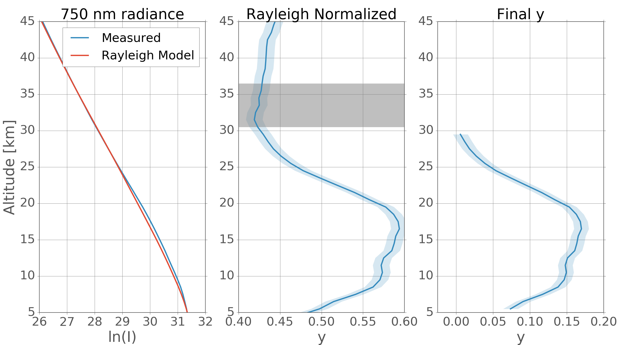
Figure 1: Panel A shows the unormalized radiance in blue, and a modelled signal assuming an atmosphere with no aerosol in red. Panel B shows the measurement normalized by the Rayleigh signal. The blue shaded region represents the measurement vector error assuming 1% noise on the radiance. The gray shaded region shows the alitudes used in the high alitude normalization. Panel C shows the final measurement vector after both Rayleigh and alitude normalizations have been applied.
Lower Bounds
Only measurements above 5km are used in the retrieval. This is the initial lower bound of the retrieval, but is raised if values of extinction greater than 0.0125 km-1 at 750nm are retrieved. If this occurs the extinction is capped at 0.0125 km-1 and the valid retrieval range is moved to the first altitude above the saturated region. These large extinction values are typical if there is a cloud in the field of view.
Ozone
Ozone is retrieved using 7 wavelength pairs in the UV and one wavelength triplet in the visible. The UV doublets are constructed from an absorbing wavlength normalized by the radiance at 350nm. The measurement vector at wavelength \(k\) and altitude \(j\) is then
where \(j_n\) is the range of altitudes used for the normalization. Similarly, the Chappius triplet is composed as
The wavelengths used in the version 1.00 retrieval are shown below.
| Measurement Vector | Wavelengths [nm] | Reference Alt [km] | |
|---|---|---|---|
| Absorbing | Reference | ||
| 1 | 292.43 | 350.31 | 59-64 |
| 2 | 302.17 | 350.31 | 55-60 |
| 3 | 306.06 | 350.31 | 51-56 |
| 4 | 310.70 | 350.31 | 48-53 |
| 5 | 315.82 | 350.31 | 46-51 |
| 6 | 322.00 | 350.31 | 42-47 |
| 7 | 331.09 | 350.31 | 39-44 |
| 8 | 602.39 | 543.84,678.85 | 30-35 |
However, it is easy expand (or reduce) the number of wavelengths and relative weights of each wavelength used in a measurement. The general form for measurement vector \(k\) is
where \(w_{lk}\) is the weight for each wavelength used to compose measurement vector \(k\).
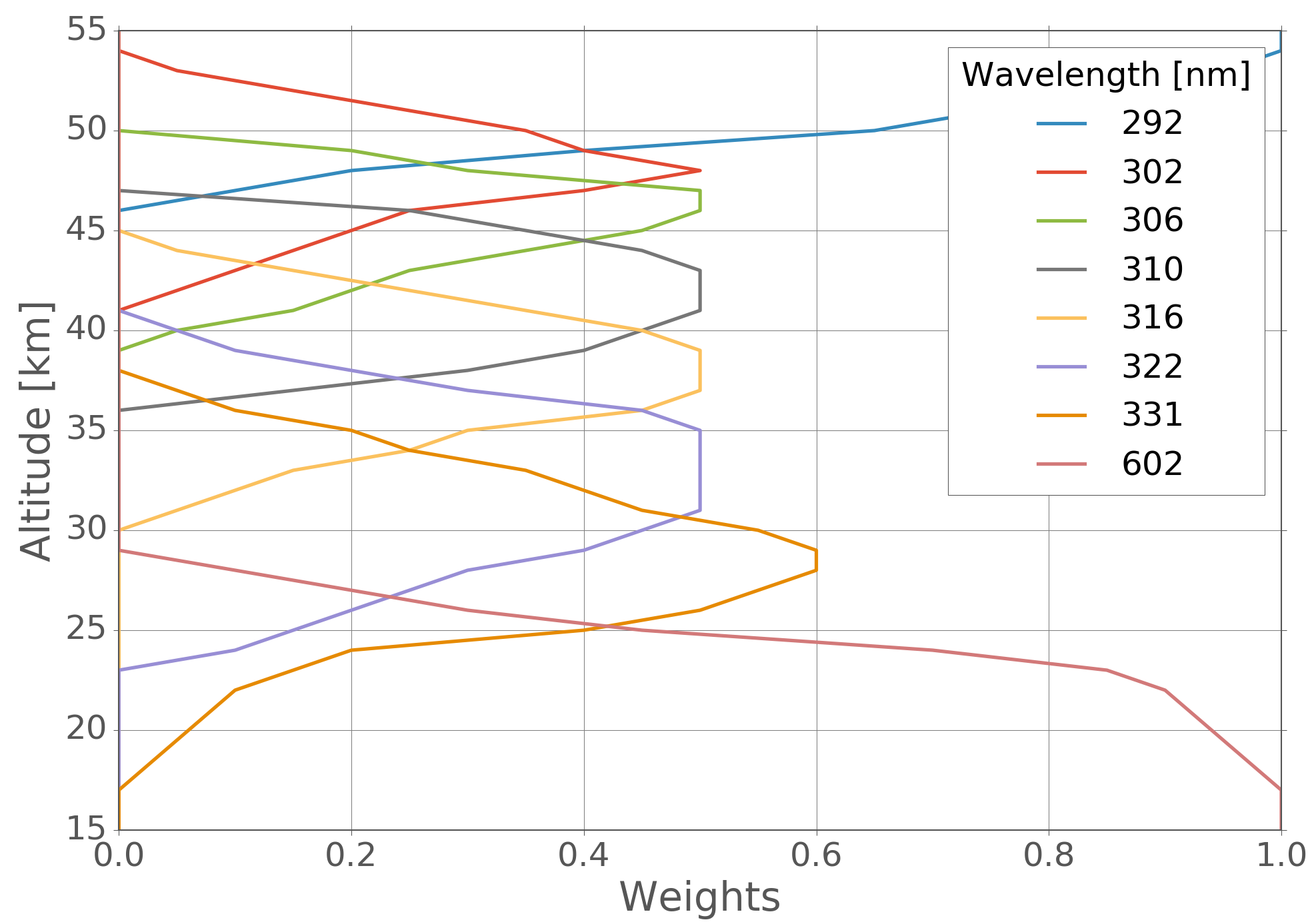
To avoid the use measurements vectors that contain wavelenths where the atmosphere is optically thick, and the radiative tranfser less robust, the measurements vectors are also weighted in the retrieval, either with \(W_{ki}\) or \(W\) for the MART and LM retrievals respectively. The default \(W_{ki}\) weights are the same as those used in [Degenstein2009], and are shown in Figure 3.
Coupled Retrieval
To couple the retrieval of the three species, they are retrieved in following order
- Albedo
- Aerosol
- Albedo
- Aerosol
- Ozone