The Platforms Model¶

The skretrieval.platforms package provides support to simulate platforms such as spacecraft, aircraft, balloons and ground-based sites. Instruments are mounted on platforms at given orientations, similar to how physical instruments are bolted on to real platforms, and the platform is positioned and rotated to collect the desired set of measurements.

Its goal within the skretrieval framework is to assist in the generation of the set of times, positions and look vectors given to The Forward Model. Users who have their own techniques for calculating positions and look vectors for the The Forward Model can continue using their own code or, if they wish, switch over to using the Platform class.

Class Platform provides access to two primary aspects,

Simulation of various platforms used in remote atmospheric sensing.

Generation of sets of platform position and orientation using various positioning and pointing techniques.

The Platform class utilizes several Control Frames and provides rotation matrices to transform between the frames. The user will typically define instrument lines of sight in the Instrument Control Frame (ICF). The instrument is optionally mounted on a platform and the platform rotated in space and time to execute the desired measurement plan. Users will normally transform the instrument look vectors to the Geocentric Control Frame (ECEF) for input to radiative transfer codes but the platform can also transform the look vector to the local geodetic control frame or platform control frame if preferred.

Class Platform provides a high level interface which can be used to calculate platform positions and orientations needed to simulate a set of measurements. The class, as provided out-of-the-box, provides access to a library of common techniques that that should meet most user needs but the API allows new techniques to be developed and added by users. The problem usually reduces into two parts,

selection of an instrument positioning technique.

selection of an instrument pointing technique.

Example¶

Consider a simulation where an instrument onboard a sun-synchronous satellite at an altitude of 600 km needs to look in the limb at a tangent point at 35 km altitude over Saskatoon, Saskatchewan, located at (52.0N, -107.0E). The observation will be made at approximately 2020-07-15 15:00 UTC. The satellite is configured so the instrument is always looking at a bearing of 45 degrees from local North at the satellite location.

We shall demonstrate three techniques that could be used to solve the problem. The three techniques are based upon significantly different algorithms but, from the user’s perspective, are implemented in an almost identical manner.

Option 1: llh¶

Use the Platform class with no special configuration. Set the time and position of the satellite with the llh positioning technique. Then configure the platform orientation with the tangent_altitude pointing technique using limb roll control so it is looking at that tangent point. This will generate the required position and look vector for the given conditions. The option has the limitation that it is difficult to choose the position of the platform so the tangent point is over Saskatoon:

from skretrieval.platforms import Platform

platform = Platform()
utc = ['2020-07-15T15:00:00.0000000']
observer = [52.0, -107.0, 600000.0]
tanpoint = [35000.0, 45.0]
platform.add_measurement_set(utc, ('llh', observer), ('tangent_altitude', 'limb', tanpoint))
opticalmeasurements = platform.make_optical_geometry()

If you want to print out the location of the satellite and the tangent point you can use the following snippet of code:

import sasktran as sk

geo = sk.Geodetic()
entry = opticalmeasurements[0]
geo.from_xyz(entry.observer)
obslat = geo.latitude
obslng = geo.longitude
obshgt = geo.altitude / 1000.0
geo.from_tangent_point(entry.observer, entry.look_vector)
tanlat = geo.latitude
tanlng = geo.longitude
tanhgt = geo.altitude / 1000.0
print('Satellite location = ({:5.2f}N,{:6.2f}E) at a height of {:6.2f} km'.format(obslat, obslng, obshgt))
print('Tangent location   = ({:5.2f}N,{:6.2f}E) at a height of {:6.2f} km'.format(tanlat, tanlng, tanhgt))

and you should get:

Satellite location = (52.00N,253.00E) at a height of 600.00 km
Tangent location   = (63.65N,291.78E) at a height of  35.00 km

The tangent point is at 35 km as requested but it is not over Saskatoon, which is not surprising as we, perhaps erroneously, put the satellite directly over Saskatoon. To get the tangent point directly over Saskatoon you could iteratively adjust the satellite position until you find teh right locations. But there is an easier way demonstrated below in option 2.

Option 2: looking_at_llh¶

The second option provides a more sophisticated technique to position the satellite so the resultant tangent point will end up above Saskatoon. In this case set the time and position of the satellite are set with the looking_at_llh positioning technique; this technique has 5 parameters that position the satellite at the requested altitude so it will have the requested tangent altitude at the requested location with the requested bearing. It then configures the platform orientation with the tangent_altitude pointing technique using limb roll control so it is looking at that tangent point:

from skretrieval.platforms import Platform

platform = Platform()
utc = ['2020-07-15T15:00:00.0000000']
observer = [52.0, -107.0, 35000.0, 45.0, 600000.0]
tanpoint = [35000.0, 45.0]
platform.add_measurement_set(utc, ('looking_at_llh', observer), ('tangent_altitude', 'limb', tanpoint))
opticalmeasurements = platform.make_optical_geometry()

Examination of the location of the satellite and tangent point using the same code as in option 1 above gives:

Satellite location = (38.23N,226.13E) at a height of 600.00 km
Tangent location = (52.02N,252.98E) at a height of  35.00 km

Now the tangent point is above Saskatoon and the satellite has been placed at a location so it is looking toward Saskatoon at a tangent altitude of 35 km and a bearing of 45 degrees. Note that the tangent point is not “exactly” above Saskatoon. It is off by approx 0.02 degrees which is due to limitations in the algorithm used.

Option 3: satellite¶

This option configures the Platform class with a sun-synchronous satellite orbit propagator. the satellite is flown along the orbit track by providing a sequence of 100 universal times at 1 minute intervals. The position of the platform is now extracted using the from_platform positioning technique while the look vector is still extracted with the tangent_altitude pointing technique and limb roll control. This option requires a bit more setup but allows the user to fly the satellite around the Earth and generate other positions and look vectors:

mjd0 = sktime.ut_to_mjd('2020-07-15T15:00:00.000000')                                                         # Define the time of the ascending node
satellite = SatelliteSunSync(mjd0,                                                                             # Create a sun-synchronous satellite
                             orbittype='sgp4',
                             period_from_altitude=600000.0,
                             localtime_of_ascending_node_hours=2.75)
platform = Platform(platform_locator=satellite)                                                                 # Create a platform which can use the sun-synchronous satellite for its position

utc = mjd0 + np.arange(0, 100) / 1440.0                                                                         # Get measurements every minute along the orbit starting at the ascending node.
looktanalt = [(35000.0, 45)]                                                                                    # Look at a tangent altitude of 35 km, at a geographic bearing of 45 degrees at the satellite location. Note, the parameter set will be expanded to N measurements
platform.add_measurement_set(utc, ('from_platform',), ('tangent_altitude', 'limb', looktanalt))                 # Add the measurement set
opticalmeasurements = platform.make_optical_geometry()

This technique has the same problem as option 1 in that it is difficult to pre-configure the satellite to fly exactly over Saskatoon with the proper geometry. However, we fiddled with the local time of the ascending node of the satellite and if you look at the 38’th entry of the 100 returned opticalmeasurement values you should see that it has a tangent point close to Saskatoon:

38 Satellite location = (38.26N,235.59E) at a height of 605.39 km
38 Tangent location   = (52.09N,262.62E) at a height of  35.00 km

Measurement Sets¶

The user must define what constitutes a set of measurements. This may be as simple as one exposure or something much more complicated such as a spatial scan of a specific atmospheric region. In our experience, we almost always break the definition of measurements sets into the following three steps,

Define (or acquire) a set of universal times at which the measurements are made.

Specify (or acquire) the position of the platform associated with each measurement at each universal time.

Specify (or acquire) the pointing of the platform associated with each measurement at each universal time.

Example¶

Configure a satellite to acquire a height profile of spectra over Saskatoon (52N, -107E) in the summer time from which atmospheric aerosols can be inferred over Saskatooon .

Option 1: A simple emulator fixes a satellite ~20 degrees south of Saskatoon at 600 km looking northwards in the limb. There will be 50 measurements scanning from 0 km to 50 km all made at the same location and same time UTC (2020-06-21T18:00:00.000000)

Option 2: A sun-synchronous satellite with an ascending node at 12:00LT will fly over Saskatoon on 2020-06-21. It will collect 50 measurements scanning from 0 to 50 km. The measurements will be one second apart.

The skretrieval.platforms package can help with both of these scenarios and the user would choose which scenario they wish to model.

Internal Representation¶

Measurement sets are internally stored within class Platform using an instance of ObservationPolicy. This class stores a set of times, position and rotation matrices used for the measurements. This information is independent of the instrument, apart from its mounting orientation, and cannot be used by retrieval and radiative transfer codes until it is converted into a set of times, positions and instrument look vectors, such as those found in OpticalGeometry.

Positioning Technique¶

Positioning Techniques are used to specify the position of a platform at a set of measurement times. For example, one technique may specify the position of a platform using a three element array of geodetic coordinates, \((latitude, longitude, height)\), while another technique may specify the same location using a three element array of geocentric coordinates, \((x,y,z)\). The user chooses which technique they wish to use, see table below.

Coding up the positioning technique consists of the following steps

Determine the number of measurements. This is driven by the number of different platform positions and orientations

Create an array of universal times with one time for each measurement. The times can be the same or they can be different

Create an array of platform position arrays. One array entry is created for each measurement.

Create a tuple whose first element identifies the position technique and the second element is the array of positions.

Pass the array of UTC times and the tuple of position technique into add_measurement_set() along with orientation info described below.

For example:

utcarray = ['2020-09-24T12:15:36.123456', '2020-09-24T12:15:37.456123', '2020-09-24T12:15:38.654321', '2020-09-24T12:15:39.654321']
posarray = [(52, -107, 600000), (53, -107, 600001), (54, -107, 600002), (55,-107, 600003)]
postechn = ('llh',posarry)
.
.
looktechn = <Various look definition statements, see below>
.
.
platform.add_measurement_set(utcarray, postechn, looktechn)

There are three positioning techniques provided with the skretrieval.platforms package. Their values are given in the table below,

Position Technique	Description
xyz	The platform is placed at the geocentric ECEF point given by (x,y,z)
llh	The platform is placed at the geodetic ECEF location given by (latitude, longitude, height)
looking_at_llh	The platform is placed so it is looking at a given location with a given geographic bearing.
from_platform	The platform is placed at the position of a real instrument or platform simulator using `PlatformLocation`.

The last entry, from_platform, allows users to fetch the platform position at a given universal time from an attached PlatformLocation object. This technique is used to model various satellite trajectories, both real and simulated, and is useful when users wish to simulate measurements as a satellite, aircraft or balloon, moves along its trajectory.

xyz¶

The xyz positioning technique places the platform at the N specified geocentric locations for each measurement in the parameter array.

( 'xyz', parameters )

parameters is an N element array of three element arrays, [array[3], array[3], ...]. It is anything that can be sensibly coerced into a numpy array of dimension (N,3). All values are expressed in meters in the Geocentric Control Frame (ECEF).

Parameters

[0] (float) – x component of the platform position.
[1] (float) – y component of the platform position.
[2] (float) – z component of the platform position.

Example:

from skretrieval.platforms import Platform

def make_geometry():
    platform = Platform()
    utc  = ['2020-09-24T12:15:36.123456',     '2020-09-24T12:15:37.456123',     '2020-09-24T12:15:38.654321',     '2020-09-24T12:15:39.654321']
    pos  = [(7223456.0,1023456.0, 1423456.0), (7523456.0,923456.0, 1523456.0)   (7223456.0,1023456.0, 1423456.0), (7523456.0,923456.0, 1523456.0)]
    look = [(35000, 10),                      (27000, 5),                       (24000, 0, 0),                    (21000, -5, 0)]

    platform.add_measurement_set( utc, ('xyz', pos), ('tangent_altitude', 'limb', look) )
    obspolicy = platform.make_observation_policy()

llh¶

The platform is placed at the geodetic location given by the three element tuple, (latitiude, longitude, height), where latitude and longitude are specified in degrees and height is specified in meters above sea-level.

( 'llh', parameters )

parameters is an N element array of three element arrays, [array[3], array[3], ...]. It is coerced into a numpy array of dimension (N,3).

Parameters

[0] (float) – Latitude. The geodetic latitude of the platform position in degrees.
[1] (float) – Longitude. The geodetic longitude of the platform position in degrees. positive East.
[2] (float) – Height. The height of the platform above sea-level in meters.

Example:

from skretrieval.platforms import Platform

def make_geometry():
    platform = Platform()
    utc  = ['2020-09-24T12:15:36.123456', '2020-09-24T12:15:37.456123', '2020-09-24T12:15:38.654321', '2020-09-24T12:15:39.654321']
    pos  = [(52, -107, 600000),           (53, -107, 600001),           (54, -107, 600002),           (55,-107, 600003)]
    look = [(35000, 10, 0),               (27000, 5, 0),                (24000, 0, 0),                (21000, -5, 0)]

    platform.add_measurement_set( utc, ('llh', pos), ('tangent_altitude', 'limb', look) )
    platform.make_complete_measurement_set()

looking_at_llh¶

The platform is placed at the location and height that allows it to view the given target tangent point along the given geographic bearing.

( 'looking_at_llh', parameters )

parameters is an N element array of five element arrays, [array[5], array[5], ...]. It is coerced into a numpy array of dimension (N,5).

Parameters

[0] (float) – Tangent Latitude. The latitude of the tangent location
[1] (float) – Tangent Longitude. The longitude of the tangent location
[2] (float) – Tangent Altitude. The height of the tangent above sea-level in meters.
[3] (float) – Geographic Bearing. The geographic bearing in degrees of the target from the observer’s location. This is calculated at the observer’s location. 0 is North, 90 is East, 180 is South and 270 is West.
[4] (float) – Observer Height. The height of the observer in meters above sea-level.

Example. In the following example a satellite is positioned so it is at 600 km altitude and is looking at a bearing of 45 degrees (NE) towards a tangent point at 10 km altitude above (52N, -107E). A line of sight is chosen so the instrument is looking in the same geographic bearing at a tangent altitude at 5 km:

from skretrieval.platforms import Platform

platform = Platform()
utc = ['2020-09-24T18:00:00.0000000']
observer = [52.0, -107.0, 10000.0, 45.0, 600000.0]
tanpoint = [5000.0, 45.0]
platform.add_measurement_set(utc, ('observer_looking_at_llh', observer), ('tangent_altitude', 'limb', tanpoint))
obspolicy = platform.make_observation_policy()

from_platform¶

The platform is placed at the position returned by a call to update_position() for the universal time of each measurement. The user must configure class Platform to use the appropriate derived instance of class PlatformLocation class that meets their needs.

( 'from_platform', ) or ('from_platform'): No parameters are required. Parameters can be passed in but are ignored.

Example:

from skretrieval.platforms import Platform

def make_geometry():
    platform = Platform()
    utc  = ['2020-09-24T12:15:36.123456', '2020-09-24T12:15:37.456123', '2020-09-24T12:15:38.654321', '2020-09-24T12:15:39.654321']
    look = [(35000, 10, 0),               (27000, 5, 0),                (24000, 0, 0),                (21000, -5, 0)]
    platform.add_measurement_set( utc, ('from_platform',), ('tangent_altitude', 'limb', look) )
    obs_policy = platform.make_observation_policy()

Roll Control¶

Full specification of the platform orientation in space requires the roll of the instrument \(\hat{z}_{ICF}\) axis around the instrument \(\hat{x}_{ICF}\) axis. The skretrieval.orientation_techniques package uses of three methods to determine the location of zero roll, see table below. Each definition has been chosen so the default value of 0.0 corresponds to the value normally chosen for that class of simulations.

Roll Control Setting	Description
limb	Limb observations: the zero point of roll is parallel to local up at the tangent point.
nadir	Nadir observations: the zero point of roll is parallel to local north at the given point.
standard	Aircraft, balloon, ground site: the zero point of roll is parallel to local up at the observer location.

Roll is always measured clockwise when looking along the look vector from the observer’s position, i.e. the +Z instrument axis rotates towards the -Y direction, similar to the roll definition used in aircraft systems.

The roll control value, if required, is provided as one of the parameters given in each pointing technique declaration and many pointing techniques allow you to omit the value and assume the default value of 0.0.

limb¶

The limb roll control setting is typically used for limb viewing geometries. This setting defines the point of zero roll as the point where the instrument \(\hat{y}_{ICF}\) axis is aligned with the horizon at the tangent point. This is determined by aligning the instrument \(\hat{z}_{ICF}\) with the vertical unit vector at the tangent point. This ensures the instrument \(\hat{y}_{ICF}\) axis is parallel to the horizon and points to the portside of the boresight.

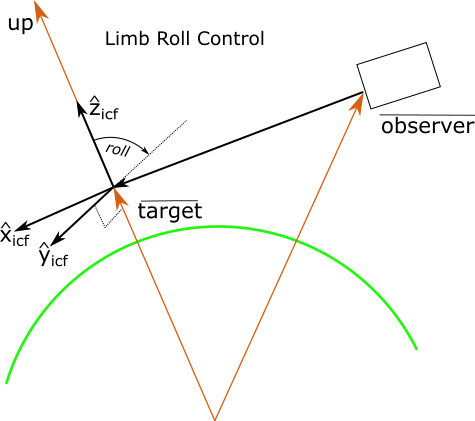
Limb control aligns instrument \(\hat{z}_{ICF}\) with the up unit vector at the tangent point¶

The limb roll control setting is not meaningful for several scenarios. For example, look directions that are straight down have poorly defined horizons and result in definitions which at best are not sensible. Similarly look vectors that point upwards only have tangent points that are behind the observer and this, again, results in definitions which are not sensible.

The OrientationTechniques class will reject all measurement states with the limb roll control setting if the target tangent point is above the observer’s position or is below 5000 meters below the surface of the Earth.

nadir¶

The nadir roll control setting is typically used for nadir viewing geometries. This setting defines the point of zero roll as the point where the instrument \(\hat{z}_{ICF}\) axis is aligned with geographic North at the target point. It is determined by rotating the instrument \(\hat{z}_{ICF}\) axis around the boresight, \(\hat{x}_{ICF}\), until the boresight, the North unit vector and the instrument \(\hat{z}_{ICF}\) are all co-planar with \(\hat{z}_{ICF}\) co-aligned with North. This ensures the instrument \(\hat{y}_{ICF}\) axis is parallel to the horizon and points to the portside of the boresight.

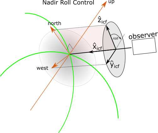
nadir control aligns instrument \(\hat{z}_{ICF}\) with the North unit vector at the nadir target point¶

The nadir roll control setting is not meaningful for several scenarios. For example, look directions that are horizontal are poorly defined nadir geometries and result in definitions which, at best, are not sensible. Similarly look vectors that point upwards only have nadir points that are behind the observer and this, again, results in definitions which are not sensible.

standard¶

The standard roll control setting is typically used for ground-based sites, aircraft and balloons. The standard setting defines the point of zero roll as the point where the instrument \(\hat{y}_{ICF}\) axis is in the horizontal plane at the observer’s location. It is determined by rotating the instrument \(\hat{z}_{ICF}\) axis around the boresight, \(\hat{x}_{ICF}\), until the boresight, the up unit vector and the instrument \(\hat{z}_{ICF}\) are all co-planar with \(\hat{z}_{ICF}\) co-aligned with up.

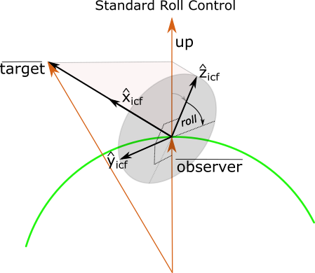
standard roll control places the instrument \(\hat{y}_{ICF}\) axis in the horizontal plane of the observer.¶

The standard roll control setting is sensible but has the unfortunate property that it is ill-conditioned for look vectors which are straight up or down as all roll values place \(\hat{y}_{ICF}\) in the horizontal plane. To assist with this issue, the code allows orientation techniques to specify a horizontal unit vector which is derived from azimuth or yaw parameters passed in from the user. If the specific orientation technique does not provide hints about the horizontal vector then OrientationTechniques will choose the North direction as the reference horizontal direction for all look vectors. This latter option is not optimal as it results in abrupt changes in roll configuration at angles within ~0.5 degrees of vertical.

Pointing Technique¶

Pointing techniques are used to rotate the Platform Control Frame (PCF) so the instrument boresight, given by the \(\hat{x}_{ICF}\) unit vector in the Instrument Control Frame (ICF), is pointing toward the desired target. We have provided a common set of techniques to orient the platform. The orientation techniques only modify the platform rotation matrix. This allows users to define as many look vectors as they wish in the Instrument Control Frame (ICF) and rotate them all, in a consistent fashion, to the final reference frame with the boresight looking at the target location.

Pointing techniques are only intended to provide a convenient method of specifying look vectors and users are free to develop their own solutions if they wish. We provide techniques to support common geometries encountered in atmospheric remote sensing, limb, nadir and standard. The various techniques are summarized in the table below. Note that we recommended the Roll Control setting to be used with each technique but this is only a guideline and users may choose to use other Roll Control values if it meets their needs. This list of techniques is not extensive by any means and we have built the OrientationTechniques class so the new techniques can be added as needs arise, including techniques developed by users.

Pointing Technique	Recommended Roll Control	Description
tangent_xyz_look	limb	Look towards a tangent point with an (x,y,z) unit vector.
tangent_altitude	limb	Look towards a tangent point with given height and geographic bearing
location_xyz	nadir	Look in nadir towards location given by x,y,z
location_llh	nadir	Look in nadir towards location at geodetic lat, long, height.
from_platform	—	Set platform orientation from :class`~.Platform` class. This is used for real instruments
unit_vectors	—	Set platform orientation with explicit \(\hat{x}_{ICF}\) and \(\hat{z}_{ICF}\) unit vectors.
azi_elev	standard	Look in azimuth, elevation and roll direction.
yaw_pitch_roll	standard	Look in yaw, pitch, roll direction
tangent_from_orbitplane	limb	Look towards a tangent point with a given height and bearing from the orbit plane.

Extreme Cases

It is difficult to provide sensible analysis for extreme cases. For example, the roll control zero point is undefined in limb mode when looking directly downwards. Similar conditions occur when looking horizontally in nadir mode. The software does detect these extreme conditions and attempts to do something reasonable but we strongly recommend the user only use limb and nadir roll control values for sensible and nadir geometries.

The standard setting has difficulties when looking straight up or down if used with techniques intended for nadir or limb geometries as the required azimuth of the instrument \(\hat{y}_{ICF}\) becomes undefined. The problem does not exist for the techniques specifically recommended for standard roll control as we ensure the users explicitly provides the azimuth information.

tangent_xyz_look¶

Configures the platform so the instrument boresight, \(\hat{x}_{ICF}\), points in the specified look direction. The tangent point of the look vector is used as the target location for determining Roll Control in either limb or nadir modes.

( 'tangent_xyz_look', roll_control, parameters )

parameters is an N element array of 3 or 4 element arrays, [array[3], array[3], ...] or [array[4], array[4], ...]. It is anything that can be sensibly coerced into a numpy array of dimension (N,3) or (N,4). All look vectors are expressed in the Geocentric Control Frame (ECEF)

Parameters

roll_control (str) – The Roll Control value applied to this set of measurements. Most users will use limb.
[0] (float) – x. The x component of the look direction unit vector
[1] (float) – y. The y component of the look direction unit vector
[2] (float) – z. The z component of the look direction unit vector
[3] (float) – roll. Optional [default 0.0]. The roll angle in degrees of the instrument control frame around the boresight, \(\hat{x}_{ICF}\), from the zero point implied by roll_control

Example:

def configure_look( platform: Platform ):
    utc  = ['2020-09-24T12:15:36.123456', '2020-09-24T12:15:37.456123', '2020-09-24 12:15:38.654321']
    pos  = [(52, -107, 600000), (52, -107, 600000), (54, -107, 600002)]
    look = [(0.58311235, -0.43069497, -0.68882642,  0.0), ( 0.58320668, -0.43220012, -0.68780304, 0.0), (0.5833907, -0.43522548, -0.68573615, 0.0)]

    platform.add_measurement_set('limb', utc, ('llh', pos), ('tangent_xyz_look', 'limb', look))
    obspolicy = platform.make_observation_policy()

Note

This technique is intended to be used for tangent altitudes that are below the observer’s position and above 5 km below sea-level. Look vectors outside this range are discarded.

tangent_altitude¶

The platform looks at the tangent height, geographic bearing and roll specifie in the parameters. This technique should be used to get the instrument boresight look

( 'tangent_altitude', roll_control, parameters )

parameters is an N element array of 2 or 3 element arrays, [array[2], array[2], ...] or [array[3], array[3], ...]. It is anything that can be sensibly coerced into a numpy array of dimension (N,3) or (N,4).

Parameters

roll_control (str) – The Roll Control value applied to this set of measurements. Most users will use limb.
[0] (float) – height. The height in meters above sea-level of the requested tangent altitude. This value should be less than the observers height and greater than 5 km below ground.
[1] (float) – bearing. The geographic, compass bearing in degrees of the tangent direction measured at the observer’s location. 0 is North, 90 is East, 180 is South and 270 is West.
[2] (float) – roll. Optional [default 0.0]. The roll angle in degrees of the instrument control frame around the boresight, \(\hat{x}_{ICF}\), from the zero point implied by roll_control

tangent_from_orbitplane¶

The platform looks at the tangent height, bearing and roll specified in the parameters. The bearing is measured from the orbit plane rather than geographic North. This technique is only available on platforms that have a valid platform_locator object which calculates velocity in addition to position.

( 'tangent_from_orbitplane', roll_control, parameters )

parameters is an N element array of 2 or 3 element arrays, [array[2], array[2], ...] or [array[3], array[3], ...]. It is anything that can be sensibly coerced into a numpy array of dimension (N,3) or (N,4).

Parameters

roll_control (str) – The Roll Control value applied to this set of measurements. Most users will use limb.
[0] (float) – height. The height in meters above sea-level of the requested tangent altitude. This value should be less than the observers height and greater than 5 km below ground.
[1] (float) – bearing. The bearing in degrees of the tangent point from the orbit plane. The forward looking direction, parallel to the platform velocity is the point of zero bearing. Bearing increases in the same direction as a compass bearing, i.e. clockwise when viewed from above: North->East->South->West.
[2] (float) – roll. Optional [default 0.0]. The roll angle in degrees of the instrument control frame around the boresight, \(\hat{x}_{ICF}\), from the zero point implied by roll_control

Note

The platform_locator can be set when you create an instance of class Platform.

location_xyz¶

The platform looks at the given geocentric location (x,y,z) with roll of ‘roll’ degrees. Typically used for satellite nadir observations

( 'location_xyz', roll_control, parameters )

parameters is an N element array of 3 or 4 element arrays, [array[3], array[3], ...] or [array[4], array[4], ...]. It is anything that can be sensibly coerced into a numpy array of dimension (N,3) or (N,4). All position vectors are expressed in meters in the Geocentric Control Frame (ECEF)

Parameters

roll_control (str) – The Roll Control value applied to this set of measurements.
[0] (float) – x. The x component of the target position vector
[1] (float) – y. The y component of the target position vector
[2] (float) – z. The z component of the target position vector
[3] (float) – roll. Optional [default 0.0]. The roll angle in degrees of the instrument control frame around the boresight, \(\hat{x}_{ICF}\), from the zero point implied by roll_control

location_llh¶

The platform looks at the given geodetic location (lat, lng, height) with roll of ‘roll’ degrees. Typically used for satellite nadir observations

( 'location_llh', roll_control, parameters )

parameters is an N element array of 3 or 4 element arrays, [array[3], array[3], ...] or [array[4], array[4], ...]. It is anything that can be sensibly coerced into a numpy array of dimension (N,3) or (N,4). All position vectors are expressed in meters in the Geocentric Control Frame (ECEF)

Parameters

roll_control (str) – The Roll Control value applied to this set of measurements.
[0] (float) – Latitude. The geodetic latitude of the target position in degrees.
[1] (float) – Longitude. The geodetic longitude of the target position in degrees
[2] (float) – Height. The height of the target position above sea-level in meters.
[3] (float) – roll. Optional [default 0.0]. The roll angle in degrees of the instrument control frame around the boresight, \(\hat{x}_{ICF}\), from the zero point implied by roll_control

azi_elev¶

The platform looks in the direction given by azimuth, elevation and roll (applied in that order). Used for ground sites

( 'azi_elev', roll_control, parameters )

parameters is an N element array of 2 or 3 element arrays, [array[2], array[2], ...] or [array[3], array[3], ...]. It is anything that can be sensibly coerced into a numpy array of dimension (N,2) or (N,3).

Parameters

roll_control (str) – The Roll Control value applied to this set of measurements.
[0] (float) – Azimuth. The geographic azimuth of the instrument boresight in degrees from North. Measured clockwise from North. 0 is North, 90 is East, 180 is South, 270 is West.
[1] (float) – Elevation. The elevation in degrees of the instrument boresight from the horizontal plane at the observer’s location. Positive elevation (0-90) is upwards. Negative elevation (-90 to 0) is downwards.
[2] (float) – roll. Optional [default 0.0]. The roll angle in degrees of the instrument control frame around the boresight, \(\hat{x}_{ICF}\), from the zero point implied by roll_control. Most users will use standard.

yaw_pitch_roll¶

The platform applies pointing information in the order yaw, pitch, roll. This is useful for aircraft and balloon systems. Most users will choose to use standard Roll Control.

( 'yaw_pitch_roll', roll_control, parameters )

parameters is an N element array of 2 or 3 element arrays, [array[2], array[2], ...] or [array[3], array[3], ...]. It is anything that can be sensibly coerced into a numpy array of dimension (N,2) or (N,3).

Parameters

roll_control (str) – The Roll Control value applied to this set of measurements.
[0] (float) – Yaw. The geographic bearing of the instrument boresight in degrees from North. Measured clockwise from North. 0 is North, 90 is East, 180 is South, 270 is West.
[1] (float) – Pitch. The pitch or elevation elevation in degrees of the instrument boresight from the horizontal plane at the observer’s location. Positive elevation (0-90) is upwards. Negative elevation (-90 to 0) is downwards.
[2] (float) – roll. Optional [default 0.0]. The roll angle in degrees of the instrument control frame around the boresight, \(\hat{x}_{ICF}\), from the zero point implied by roll_control. Most users will use standard.

from_platform¶

The platform orientation is set by the parameters returned by the :class`~.Platform` class at the required times. This is used for real instruments

( 'from_platform',) or ('from_platform'): No limb control values or parameters are required.

unit_vectors¶

The platform orientation is explicitly so the instrument \(\hat{x}_{ICF}\) and \(\hat{z}_{ICF}\) are positioned along the two unit-vectors defined by the 6 parameters. The orientation of \(\hat{y}_{ICF}\) is given by forming a right-handed orthogonal system. The roll_control value is ignored. Users should be careful as no checks are made to ensure the input vectors are orthogonal unit vectors.

( 'unit_vectors', roll_control, parameters )

parameters is an N element array of 6 element arrays, [array[6], array[6], ...]. It is anything that can be sensibly coerced into a numpy array of dimension (N,6).

Parameters

roll_control (str) – This parameter is ignored.
[0] (float) – Xx. The x component of \(\hat{x}_{ICF}\) in the Geocentric Control Frame (ECEF)
[1] (float) – Xy. The y component of \(\hat{x}_{ICF}\) in the Geocentric Control Frame (ECEF)
[2] (float) – Xz. The z component of \(\hat{x}_{ICF}\) in the Geocentric Control Frame (ECEF)
[0] – Zx. The x component of \(\hat{z}_{ICF}\) in the Geocentric Control Frame (ECEF)
[1] – Zy. The y component of \(\hat{z}_{ICF}\) in the Geocentric Control Frame (ECEF)
[2] – Zz. The z component of \(\hat{z}_{ICF}\) in the Geocentric Control Frame (ECEF)

Platform Class¶

class skretrieval.platforms.Platform(observation_policy: Optional[skretrieval.platforms.platform.observationpolicy.ObservationPolicy] = None, platform_locator: Optional[skretrieval.platforms.platform.platformlocator.PlatformLocation] = None)¶

The purpose of the Platform class is to capture the details of the physical platform carrying an instrument. Common examples of platforms used in atmospheric research are spacecraft, aircraft, balloons and ground-based sites. There are a myriad of details surrounding real platforms but the Platform class’s only concern is to generate a list of instrument time, location and rotation matrices that properly orient Instrument Control Frame (ICF) for each simulated measurement. This list of platform state information is internally generated and then passed onto the next stage of analysis or retrieval.

The general form of usage is to perform the following steps,

Optional. Specify how an instrument is mounted on the platform. This defines the Instrument Control Frame (ICF).
Specify the universal times for a set of measurements
Specify the position of the platform for a set of measurements using a variety of positioning techniques, see Positioning Technique and add_measurement_set()
Specify the orientation of the platform for a set of measurements using a variety of orientation techniques, see Pointing Technique and add_measurement_set().
The orientations define the Platform Control Frame (PCF) and the positions define the Geodetic Control Frame (GCF).
Create the internal ObservationPolicy for the measurement set, see make_observation_policy().
Convert the ObservationPolicy to arrays of position and instrument look vectors suitable for retrieval code.

add_current_platform_state() → int¶

Fetches the current platform position and orientation and uses this as a new sample in the observation policy.

Returns: The number of samples in the current observation policy
Return type: int

add_measurement_set(utc, observer_definitions, pointing_definitions, instrument_internal_rotation=None)¶

Adds a set of N measurements definitions to the internal list of measurement sets. An overview of position and orientation techniques is given in The Platforms Model.

Parameters

utc (Array, sequence or scalar of string, float, datetime or datetime64) – The set of universal times for the set of measurements. The array should be an array or sequence of any type that can be coerced by package sktime into a numpy array (N,) of datetime64. This includes strings, datetime, datetime64. Floating point values are also converted and are assumed to represent modified julian date. The number of universal time values defines the number of measurements in this set unless it is a scalar. In this case the time value is duplicated into an array with the same number of measurements as parameter observer_positions. All elements of the array should be of the same type and should represent universal time. Be wary of using datetime objects with explicit time-zones.
observer_positions (Tuple[str, sequence]) – A two element tuple. The first element specifies the Positioning Technique to be used to position the platform. The second element of the tuple is an array of arrays of float. The array of arrays can be any Python, list of lists, tuples or arrays that can be coerced into a two dimensional array of shape (N, numparams) where N is the number of measurements and must match the size of the utc parameter parameters and numparams is the number of parameters required by the chosen Positioning Technique. The second element of the tuple can be dropped if the positioning technique is from_platform.
look_vectors – A three element tuple. The first element of the tuple is a string that specifies the Pointing Technique. The second element of the tuple specifies Roll Control and the third element is an array of arrays of float. The array of arrays can be any Python, list of lists, tuples or arrays that can be coerced into a two dimensional array of shape (N, numparams) where N is the number of measurements and must match the size of the utc parameter and numparams is the number of parameters required by the chosen Pointing Technique
instrument_internal_rotation – Optional. An array that specifies the internal rotation of the instrument within the Instrument Control Frame (ICF). This is intended to provide support for tilting mirrors and turntables attached to the instrument that redirect the instrument boresight independently of the platform. The array specifies the azimuth, elevation and roll of the instrument boresight in the Instrument Control Frame (ICF). The array is a sequence or array that can be sensibly coerced into an array of size (N,2) or (N,3) where N is the number of measurements. N can be 1 in which case the array size is broadcast to match the number of measurements inferred from the other parameters. Elements [:,0] is the azimuth in degrees of the instrument boresight in the instrument control frame, left handed rotation around \(\hat{z}_{ICF}\). Elements [:,1] are the elevation in degrees of the instrument boresight in the instrument control frame, left handed rotation around the rotated \(\hat{y}_{ICF}\) axis. Elements[:,2], which are are optional, are the roll of the instrument boresight in degrees, right handed rotation around the rotated \(\hat{x}_{ICF}\) axis. The roll defaults to 0.0 if not supplied.

clear_states()¶: Clears all of the internally cached measurement states. This should be called when re-using a platform object to create a new measurement set.

icf_to_ecef(los_icf: numpy.ndarray) → numpy.ndarray¶

Returns the lines of sight in geographic geocentric ECEF coordinates of the lines of sight specified in the instrument control frame.

Parameters: los_icf (np.ndarray( 3,Nlos)) – A 2-D array of N unit vectors expressed in the instrument control frame
Returns: A numpy array is returned with the 3 element geographic, geocentric, line of sight unit vector for each input lines of sight and each time in the current observation set.
Return type: np.ndarray (3,Nlos, Ntime)

property icf_to_ecef_rotation_matrices¶

Returns the platform rotation matrices, one matrix for each RT calculation

Returns: The X,Y,Z icf_to_ecef_rotation_matrices of the platform.
Return type: np.ndarray(3,N)

make_observation_policy() → skretrieval.platforms.platform.observationpolicy.ObservationPolicy¶: Takes all the measurements from previous calls to add_measurement_set() and converts them into a list of measurements stored inside the internal instance of ObservationPolicy object. This list of measurements can be converted to other formats, such as OpticalGeometry required by other parts of the skretrieval package. This method clears all the measurements that have been previously added.

make_optical_geometry() → List[skretrieval.core.OpticalGeometry]¶: Takes all the measurements from previous calls to add_measurement_set() and returns them as a list of OpticalGeometry values which can be used by various retrievals. The internal ObservationPolicy is also created at this time using method make_observation_policy().

property numsamples¶

Returns the number of samples/exposures in the current observation set

Returns: The number of samples in the current observation set
Return type: int

property observation_policy¶

Returns the current internal ObservationPolicy object.

Returns: Returns the current internal ObservationPolicy object.
Return type: ObservationPolicy

property platform_ecef_positions¶

Returns the position of the platform for each RT calculation

Returns: The X,Y,Z location of the platform for each RT calculation. The coordinates are in meters form the center of the Earth,
Return type: np.ndarray(3,N)

property platform_locator¶: Sets and gets the internal PlatformLocation object. This field is set to None by default but can be set to a valid class if the user wishes to use a specialized class to get the platform position or orientation as a function of time.

property platform_pointing¶: Gets the internal PlatformPointing object. This object manages all the rotation matrices used to transform between various frames.

Satellite Classes¶

Satellite classes are used to locate the position of a platform. They are derived from class PlatformLocation. General usage of the satellite classes is as follows,

Create a specific instance of a satellite.

Update the satellite state vector to a given instant in time, see update_position()

Get the satellite position, see position(), earth_location() or lat_lon_height()

Repeat steps 2 and 3.

for example:

dt      = timedelta(minutes=1.0)                                        # step time of our simulation is one minute
numtimes= 1440                                                          # Simulate for 1 day = 1440 * one minute
platform_utc     = datetime(2019,7,26, hour =20, minute=15, second=00)           # start time of our simulation
sat     = SatelliteSunSync(  platform_utc,                                       # Create the satellite
                            orbittype='sgp4',
                            period_from_altitude=600000.0,
                            localtime_of_ascending_node_hours=18.25)

answers = np.zeros( [3, numtimes])                                      # make an array to hold the latitude, longitude, altitude of each satellite at each simulation step
times   = np.zeros( [numtimes], dtype = 'datetime64[us]')               # make an array to hold the UTC time of each simulation step.
for i in range(numtimes):                                               # for each time step
    tnow =platform_utc + i*dt                                                    # get the next time step
    times[i] = tnow                                                     # save the time of the step
    sat.update_position(tnow)                                           # Update the satellite position
    answers[:,i] = sat.lat_long_height                                  # convert XYZ position and save

The Platforms Model¶

Example¶

Option 1: llh¶

Option 2: looking_at_llh¶

Option 3: satellite¶

Measurement Sets¶

Example¶

Internal Representation¶

Positioning Technique¶

xyz¶

llh¶

looking_at_llh¶

from_platform¶

Roll Control¶

limb¶

nadir¶

standard¶

Pointing Technique¶

tangent_xyz_look¶

tangent_altitude¶

tangent_from_orbitplane¶

location_xyz¶

location_llh¶

azi_elev¶

yaw_pitch_roll¶

from_platform¶

unit_vectors¶

Platform Class¶

Satellite Classes¶

More Details¶