Diffraction Gratings

Single or multi-slit diffraction grating systems use a narrow slit located at the focus of the front-end optics to illuminate a diffraction grating with a collimated beam of light centered around the boresight direction. Diffracted light is dispersed in the direction parallel to the short edge of the slit and imaged onto the detector plane. The slit acts as an approximate delta function in the spatial dimension allowing spectral information to replace the spatial information that would have been displayed if the slit were not present. Pure monochromatic planar waves separated by a small incidence angle, \(\Delta\Omega\), at the front aperture will be separated by a small distance, \(\Delta\lambda_z\) in the detection plane. Two planar waves that are incident at the front aperture at the same angle but separated by a small change in wavelength, \(\Delta\lambda\), will also be separated by a small distance, \(\Delta\lambda_z\) in the detection plane.

We add an extra coordinate label in the detection plane in addition to the standard \((y,z)\) cartesian notation. The extra coordinate is parallel to \(z\) and is labelled as \(\lambda_z\). It is used to emphasize the relationship with the wavelength along this axis. A simple mapping relationships is established between \(\lambda_z\) and other the \(z\) variable:

\[\lambda_z = a_1(\lambda_0) + a_2(\lambda_0)\,z\]

where \(\lambda_{z}\) expresses (vertical) position on the detection plane using a wavelength scale; note that \(\lambda_0\) is described below. The wavelength scale on the detection plane is further refined as the scale is slightlyWe also define two extra wavelength labels, described in the table below, used to differentiate between on-axis andf off-axis wavelength scales.

Entity	Description
\(\lambda_z\)	The wavelength axis on the detection plane in units of wavelength (e.g. nm)
\(\lambda_0\)	Wavelength scale on the detection plane due to on-axis plane waves
\(\lambda_\Omega\)	Wavelength scale on the detection plane due to off-axis plane waves

The off-axis wavelength scale is related to the on-axis through a vertical shift.

(1)\[\lambda_\Omega = \lambda_0 + b_{\lambda_0}\Omega\]

and simply reflects that off-axis spectra are slightly offset from on-axis spectra.

Background Theory

In this section we develop the theory for the integrated signal observed in pixelated area on the detection plane.

Fig. 7 Resolution is controlled by (i) the spectral response function of the grating, (ii) the finite width of the slit and (iii) the finite width of the pixelated area

The resolution of the grating system is controlled by the convolution of three parts,

1. The grating system has an intrinsic spectral response function called the grating function. This can be derived from first principles using the number of grooves on the grating and the optical aberrations within the system or it may be provided as an empirical curve which is typically, Gaussian-like, in nature.

2. The narrow slit which acts as an approximation to a delta-function allows a finite range of incoming spatial angles to be transmitted by the system. This results in a convolution in the \(\lambda_z\) direction on the detection plane. This function is typically similar to a box-car distribution.

3. The finite size of the pixelated area in the detection plane results in a integral in the spectral dimension which is also similar to a box-car distribution.

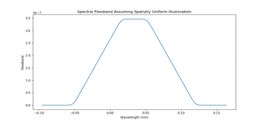
Fig. 8 Example SRF from the convolution of grating response, slit shape and pixel size

Grating Function, G

The grating function is the response of the grating and optics in the detection plane to monochromatic plane waves with a wavelength between \(\lambda_0\) and \(\lambda_0 + \Delta\lambda_0\), which is incident at the front-end optics from a fixed direction between \(\Omega\) and \(\Omega + \Delta\Omega\).

The area of the distribution is normalized to unity to ensure that photons are conserved when distributed across the detection plane (i.e. the photo must land somewhere).

The grating function may often be represented by a normalized Gaussian distribution, .. math:

G(\lambda, \lambda_\Omega) =  G(\lambda - \lambda_\Omega) = \frac{1}{\sqrt{2\pi}\sigma}e^{- \frac{(\lambda-\lambda_\Omega)^2}{2\sigma^2}}

The differential irradiance observed at the infinitessimal area between \((y,z)\) and \((y+\Delta y,z+\Delta z)\) of a pixelated region due to all wavelengths incident from directions between \(\Omega\) and \(\Omega+\Delta\Omega\) is given by,

\[e(\Omega,y,\lambda_z)\,\Delta\Omega\,\Delta y\,\Delta z = \left[ \int_{\lambda_0} R(\lambda_0, \Omega)\,G( \lambda_z - \lambda_{\Omega})\, \mathrm{d}\lambda_0\right]\,\Delta\Omega\,\Delta y\,\Delta z\]

where we have used the on-axis wavelength scale, \(\lambda_0\), as the true wavelength scale for integration purposes. We can account for the offset of the wavelength scale of inclined angles using (1) to get,

\[e(\Omega,y,\lambda_z)\,\Delta\Omega\,\Delta y\,\Delta z = \left[ \int_{\lambda_0} R(\lambda_0, \Omega)\,G( \lambda_z - \lambda_0 - b_{\lambda_0}\Omega) \, \mathrm{d}\lambda_0\right]\,\Delta\Omega\,\Delta y\,\Delta z\]

Slit Function, L

The slit function, \(L(\Omega)\), accounts for the finite angular size of the narrow slit. The slit function is often a rectangular box-car shape. If we continue our analysis then the differential irradiance observed at the infinitessimal area between \((y,\lambda_z)\) and \((y+\Delta y,\lambda_z+\Delta\lambda_z)\) is given by,

\[e(y,z)\,\Delta y\,\Delta z = \left[\int_\Omega L(\Omega)\,\int_{\lambda_0} R(\lambda_0, \Omega)\,G( \lambda_z - \lambda_0 - b_{\lambda_0}\Omega) \, \mathrm{d}\lambda_0\,\mathrm{d}\Omega\right]\,\Delta y\,\Delta z\]

Pixel Size

Integrating over the pixel area we then get the irradiance incident upon the pixel.

\[E(y,z) = \int_{y,z}\, \int_\Omega \int_{\lambda_0} R(\lambda_0, \Omega)\,L(\Omega)\,G( \lambda_z - \lambda_0 - b_{\lambda_0}\Omega) \, \mathrm{d}\lambda_0\,\mathrm{d}\Omega\,\mathrm{d} y\,\mathrm{d} z\]

where we note that \(\lambda_z\) is a function of \(z\) while \(b_{\lambda_0}\) may or may not be a function of \(\lambda_0\).

Filter-Based Instrument Interferogram Instruments