Basic Radiative Transfer Calculation with TIR
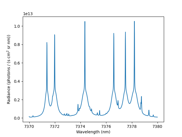
The following example demonstrates a limb radiance calculation for a methane micro window.
By importing sasktran_tir.interface, the TIR classes (engine, optical properties, and climatologies) can be accessed
without importing each class individually.
import sasktran as sk
import sasktran.tir.interface as tir
import numpy as np
import matplotlib.pyplot as plt

# select wavelengths
wavelengths = np.arange(7370, 7380, 0.01)

# create a limb line of sight
geometry = sk.VerticalImage()
# NOTE: the VerticalImage class requires sza and saa to be specified but the solar position has no effect
#       on TIR radiance calculations
geometry.from_sza_saa(sza=0, saa=0, lat=45, lon=0, tanalts_km=[20], mjd=56300, locallook=0.0)

# create an atmosphere containing methane; using the TIR engine's builtin climatologies
atmosphere = sk.Atmosphere()
atmosphere.atmospheric_state = tir.ClimatologyAtmosphericState()
atmosphere['CH4'] = sk.Species(tir.HITRANChemicalTIR('CH4'), tir.ClimatologySpecies('CH4'))

# create the engine
engine = tir.EngineTIR(geometry=geometry, atmosphere=atmosphere, wavelengths=wavelengths)

# do the calculation
radiance = engine.calculate_radiance()

# plot the result
plt.figure()
plt.plot(wavelengths, radiance)
plt.xlabel('Wavelength (nm)')
plt.ylabel('Radiance (photons / (s cm$^2$ sr nm))')

plt.show()