Air Mass Factors
The air mass factor classes are used in a way that is very similar to the weighting function classes and to the sasktran.Engine classes, but the boundaries of the box-AMF layers (box_boundaries) must be specified, and only one species can be processed at a time.
For HR and DO, the weighting functions are transformed into box-AMFs as follows:
\[A^i(\lambda) = -\dfrac{\partial\ln I(\lambda)}{\partial \tau^i(\lambda)} = -\dfrac{1}{\Delta z^i \sigma^i(\lambda)}\dfrac{1}{I(\lambda)}\dfrac{\partial I(\lambda)}{\partial n} = -\dfrac{w_{sk}^i(\lambda)}{\Delta z^i\sigma^i(\lambda)I(\lambda)}\]
where \(A^i\) is the air mass factor in the \(i^{th}\) atmospheric layer and \(w_{sk}^i(\lambda)\) is the weighting function produced by SASKTRAN and the weighting function classes.
For MC, wf_species can be set to None, in which case the box-AMFs are calculated using path length rather than path optical depth.
[1]:
import skdoas
import sasktran as sk
import numpy as np
import matplotlib.pyplot as plt

%matplotlib inline
plt.rcParams['figure.figsize'] = [15, 9]
plt.rcParams['font.size'] = 20
[2]:
# slat, slon, mjd = 52.1, -106.7, 54000.6 # Saskatoon
# mlat, mlon, mjd = 25.8, -80.2, 54000.6 # Miami
# create line of sight
observer = sk.Geodetic()
observer.from_lat_lon_alt(0., -100., 35786e3) # approximate TEMPO location
geometry = sk.NadirGeometry()
geometry.from_zeniths_and_azimuth_difference(solar_zenith=60.0, observer_zeniths=[30, 72], azimuth_differences=[60, 60])
# geometry.from_lat_lon(mjd=mjd, observer=observer, lats=[slat, mlat], lons=[slon, mlon])
# geometry.reference_point = [0.5 * (slat + mlat), 0.5 * (slon + mlon), 0., mjd]
# create atmosphere
atmosphere = sk.Atmosphere()
atmosphere.atmospheric_state = sk.MSIS90()
atmosphere['air'] = sk.Species(sk.Rayleigh(), sk.MSIS90())
atmosphere['ozone'] = sk.Species(sk.O3DBM(), sk.Labow())
atmosphere['no2'] = sk.Species(sk.NO2Vandaele1998(), sk.Pratmo())
wl = [440.]
boundaries = np.linspace(0., 6e4, 13)
# create weighting function calculators
hr_wf = skdoas.WeightingFunctionFiniteDifferenceHR(
geometry=geometry, atmosphere=atmosphere, wf_species='no2', numordersofscatter=50)
do_wf = skdoas.WeightingFunctionDO(
geometry=geometry, atmosphere=atmosphere, wf_species='no2')
mc_wf = skdoas.WeightingFunctionNullMC(
geometry=geometry, atmosphere=atmosphere, wf_species='no2',
setnumphotonsperlos=1000, numordersofscatter=50)
# pass the weighting function calculators to amf calculators
hr_amf = skdoas.AirMassFactor(hr_wf, boundaries)
do_amf = skdoas.AirMassFactor(do_wf, boundaries)
mc_amf = skdoas.AirMassFactor(mc_wf, boundaries)
# calculate the amfs
do_result = do_amf(wl).unstack('perturbation')
hr_result = hr_amf(wl).unstack('perturbation')
mc_result = mc_amf(wl).unstack('perturbation')
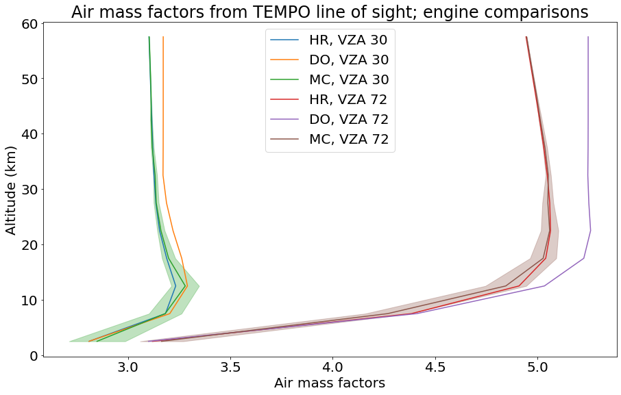
plt.plot(hr_result.amf.isel(wavelength=0, los=0), hr_result.altitude / 1e3, color='C0', label='HR, VZA 30')
plt.plot(do_result.amf.isel(wavelength=0, los=0), do_result.altitude / 1e3, color='C1', label='DO, VZA 30')
plt.plot(mc_result.amf.isel(wavelength=0, los=0), mc_result.altitude / 1e3, color='C2', label='MC, VZA 30')
plt.fill_betweenx(mc_result.altitude / 1e3, mc_result.amf.isel(wavelength=0, los=0) - mc_result.amfstd.isel(wavelength=0, los=0), mc_result.amf.isel(wavelength=0, los=0) + mc_result.amfstd.isel(wavelength=0, los=0), color='C2', alpha=0.3)
plt.plot(hr_result.amf.isel(wavelength=0, los=1), hr_result.altitude / 1e3, color='C3', label='HR, VZA 72')
plt.plot(do_result.amf.isel(wavelength=0, los=1), do_result.altitude / 1e3, color='C4', label='DO, VZA 72')
plt.plot(mc_result.amf.isel(wavelength=0, los=1), mc_result.altitude / 1e3, color='C5', label='MC, VZA 72')
plt.fill_betweenx(mc_result.altitude / 1e3, mc_result.amf.isel(wavelength=0, los=1) - mc_result.amfstd.isel(wavelength=0, los=1), mc_result.amf.isel(wavelength=0, los=1) + mc_result.amfstd.isel(wavelength=0, los=1), color='C5', alpha=0.3)
plt.title('Air mass factors from TEMPO line of sight; engine comparisons')
plt.xlabel('Air mass factors')
plt.ylabel('Altitude (km)')
plt.legend()
plt.show()
WARNING:root:the reference point set in the geometry object is ignored by EngineDO
[3]:
slat, slon, mjd = 2.1, -106.7, 54000.6 # Saskatoon
# create line of sight
observer = sk.Geodetic()
observer.from_lat_lon_alt(0., -100., 35786e3) # approximate TEMPO location
geometry = sk.NadirGeometry()
geometry.from_lat_lon(mjd=mjd, observer=observer, lats=slat, lons=slon)
geometry.reference_point = [slat, slon, 0.0, mjd]
# create atmosphere
atmosphere = sk.Atmosphere()
atmosphere.atmospheric_state = sk.MSIS90()
atmosphere['air'] = sk.Species(sk.Rayleigh(), sk.MSIS90())
atmosphere['ozone'] = sk.Species(sk.O3DBM(), sk.Labow())
atmosphere['no2'] = sk.Species(sk.NO2Vandaele1998(), sk.Pratmo())
# average atmospheric properties into constant layers:
cl_atmosphere = skdoas.utility.convert_linear_to_constant_atmosphere(
atmosphere=atmosphere,
linear_altitudes=np.linspace(0, 1e5, 201), # input atmosphere does linear interpolation on this grid
constant_altitudes=np.linspace(0, 1e5, 101), # output atmosphere has constant layers above these altitudes
reference_point=geometry.reference_point
)
wl = [440.]
boundaries = np.linspace(0., 6e4, 61)
# create weighting function calculators
hr_wf = skdoas.WeightingFunctionFiniteDifferenceHR(
geometry=geometry, atmosphere=atmosphere, wf_species='no2', numordersofscatter=1)
cl_wf = skdoas.WeightingFunctionFiniteDifferenceConstantLayersHR(
geometry=geometry, atmosphere=cl_atmosphere, wf_species='no2', numordersofscatter=1)
vg_wf = skdoas.WeightingFunctionFiniteDifferenceVariableGridHR(
geometry=geometry, atmosphere=atmosphere, wf_species='no2', numordersofscatter=1)
mc_wf = skdoas.WeightingFunctionNullMC(
geometry=geometry, atmosphere=atmosphere, wf_species='no2', numordersofscatter=1, setnumphotonsperlos=50000)
# pass the weighting function calculators to amf calculators
hr_amf = skdoas.AirMassFactor(hr_wf, boundaries)
cl_amf = skdoas.AirMassFactor(cl_wf, boundaries)
vg_amf = skdoas.AirMassFactor(vg_wf, boundaries)
mc_amf = skdoas.AirMassFactor(mc_wf, boundaries)
# calculate the amfs
hr_result = hr_amf(wl).unstack('perturbation')
cl_result = cl_amf(wl).unstack('perturbation')
vg_result = vg_amf(wl).unstack('perturbation')
mc_result = mc_amf(wl).unstack('perturbation')
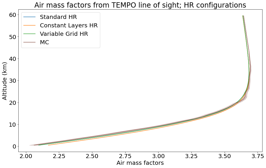
plt.plot(hr_result.amf.isel(wavelength=0, los=0), hr_result.altitude / 1e3, color='C0', label='Standard HR')
plt.plot(cl_result.amf.isel(wavelength=0, los=0), cl_result.altitude / 1e3, color='C1', label='Constant Layers HR')
plt.plot(vg_result.amf.isel(wavelength=0, los=0), vg_result.altitude / 1e3, color='C2', label='Variable Grid HR')
plt.plot(mc_result.amf.isel(wavelength=0, los=0), mc_result.altitude / 1e3, color='C5', label='MC')
plt.fill_betweenx(mc_result.altitude / 1e3, mc_result.amf.isel(wavelength=0, los=0) - mc_result.amfstd.isel(wavelength=0, los=0), mc_result.amf.isel(wavelength=0, los=0) + mc_result.amfstd.isel(wavelength=0, los=0), color='C5', alpha=0.3)
plt.title('Air mass factors from TEMPO line of sight; HR configurations')
plt.xlabel('Air mass factors')
plt.ylabel('Altitude (km)')
plt.legend()
plt.show()