Slant Column Density Retrieval

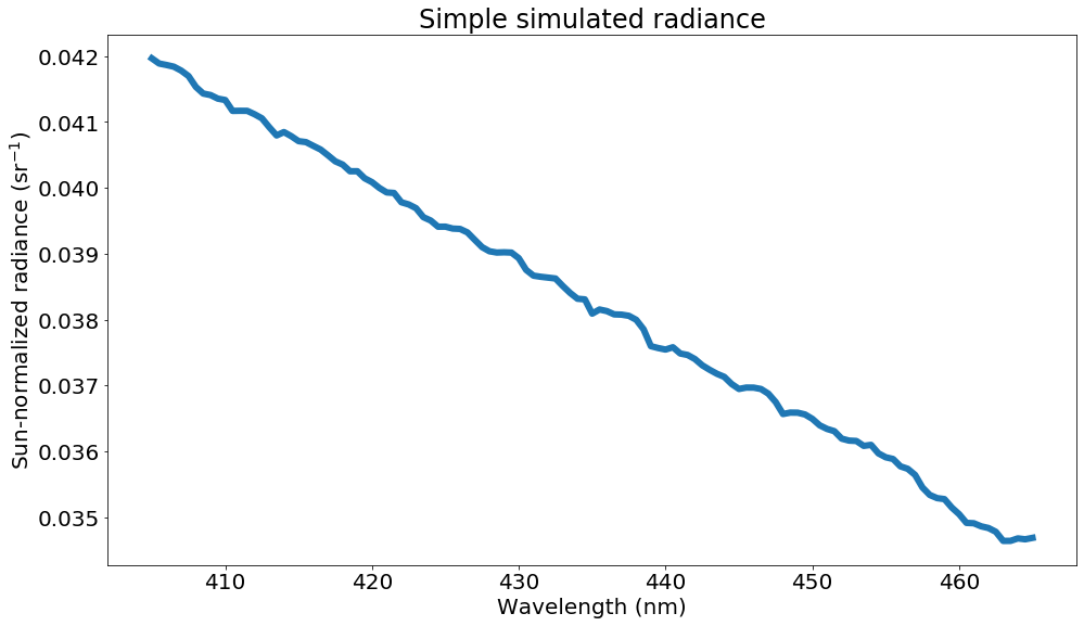
In this example, a simple nadir radiance is simulated, and the fitter is used to retrieve slant columns with and without noise.

The simulation does not include water vapour or inelastic scattering, but the fitting process includes water vapour and a Ring spectrum. As a result, the water vapour SCDs and the Ring amplitudes retrieved in this example are meaningless (and have very large retrieved uncertainties).

Simulate a simple radiance spectrum

import skdoas
import skdoas.retrieval as skr
import sasktran as sk
import numpy as np
import matplotlib.pyplot as plt
from scipy.interpolate import interp1d

%matplotlib inline
plt.rcParams['figure.figsize'] = [16, 9]
plt.rcParams['font.size'] = 20

lat, lon, mjd = 52.1, -106.7, 54000.6

# create line of sight
observer = sk.Geodetic()
observer.from_lat_lon_alt(0., -100., 35786e3)  # approximate TEMPO location
geometry = sk.NadirGeometry()
geometry.from_lat_lon(mjd=mjd, observer=observer, lats=lat, lons=lon)

# create atmosphere
atmosphere = sk.Atmosphere()
atmosphere.atmospheric_state = sk.MSIS90()
atmosphere['air'] = sk.Species(sk.Rayleigh(), sk.MSIS90())
atmosphere['ozone'] = sk.Species(sk.O3DBM(), sk.Labow())
atmosphere['no2'] = sk.Species(sk.NO2Vandaele1998(), sk.Pratmo())

# simulate a radiance spectrum
wl = np.arange(405., 465.1, 0.5)
engine = sk.EngineDO(geometry, atmosphere, wl)
rad = engine.calculate_radiance()

# store the radiance spectrum and auxiliary information in a Radiance object
measurement_l1 = skr.Radiance_SASKTRAN(
    sk_result_numpy=rad, wavelength=wl, geometry=geometry
)

plt.plot(wl, rad, linewidth=6)
plt.title('Simple simulated radiance')
plt.xlabel('Wavelength (nm)')
plt.ylabel('Sun-normalized radiance (sr$^{-1}$)')
plt.show()

Set up the fitter object and retrieve the SCDs with no noise

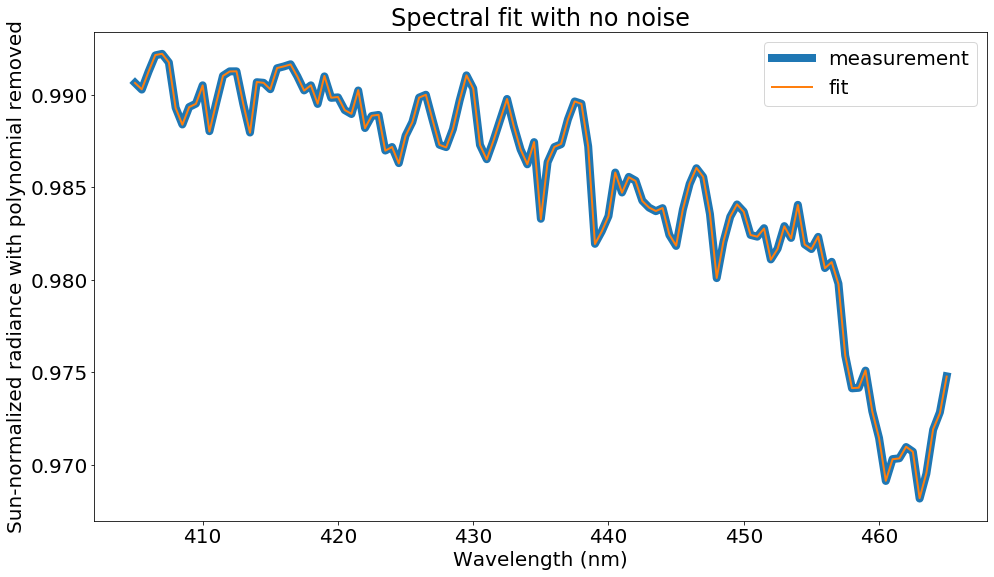
The fit is very good in this case, as identical cross sections are used for the simulation and the retrieval.

The polynomial which is part of the fitting process is removed from the radiance in the plots below in order to better display the spectral features and the quality of the fit.

When no error is supplied to the fitter, the SCD uncertainties are scaled to match the magnitude of the residual (see the documentation on absolute_sigma in https://docs.scipy.org/doc/scipy/reference/generated/scipy.optimize.curve_fit.html).

instrument = skr.DeltaFunction()
cross_sections = skr.CrossSection_Default(instrument, np.arange(405., 465.1, 0.1))
cross_sections.add_cross_section(sk.NO2Vandaele1998(), 220., 1e5)
cross_sections.add_cross_section(sk.O3DBM(), 220., 1e5)
cross_sections.add_cross_section(sk.HITRANChemical('H2O'), 220., 1e5)
cross_sections.release_weights()

solar_spectrum = skr.SolarSpectrum_Default(instrument, np.arange(405., 465.1, 0.1))
ring_spectrum = skr.RingSpectrum_Default(solar_spectrum, np.arange(405., 465.1, 0.1))

scd_object = skr.omno2.SlantColumn_OMNO2(cross_sections, ring_spectrum)
results = scd_object.fit(measurement_l1)

poly = np.polyval(scd_object.auxiliary['popt'][0][:6], wl)
plt.plot(wl, measurement_l1.radiance()[:, 0] / poly, label='measurement', linewidth=8)
plt.plot(wl, scd_object.equation(wl, *scd_object.auxiliary['popt'][0]) / poly, label='fit', linewidth=2)
plt.title('Spectral fit with no noise')
plt.xlabel('Wavelength (nm)')
plt.ylabel('Sun-normalized radiance with polynomial removed')
plt.legend()
plt.show()

print(f"no2 scd: {scd_object.auxiliary['scd_no2'][0]:.2e} +/- {scd_object.auxiliary['scd_no2_one_sigma'][0]:.2e} cm^-2")
print(f"o3 scd:  {scd_object.auxiliary['popt'][0][7]:.2e} +/- {np.sqrt(scd_object.auxiliary['pcov'][0][7, 7]):.2e} cm^-2")
print(f"h2o scd:  {scd_object.auxiliary['popt'][0][8]:.2e} +/- {np.sqrt(scd_object.auxiliary['pcov'][0][8, 8]):.2e} cm^-2")
print(f"ring amplitude:  {scd_object.auxiliary['popt'][0][9]:.2e} +/- {np.sqrt(scd_object.auxiliary['pcov'][0][9, 9]):.2e} cm^-2")

no2 scd: 1.40e+16 +/- 1.28e+13 cm^-2
o3 scd:  6.19e+19 +/- 6.15e+16 cm^-2
h2o scd:  -8.30e+19 +/- 6.48e+19 cm^-2
ring amplitude:  1.09e+22 +/- 1.10e+22 cm^-2

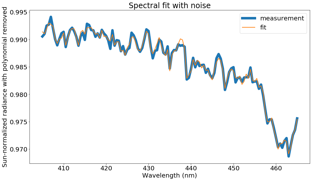
Add noise to the radiance and retrieve the SCDs

Since the added noise exactly matches the provided error, this retrieval should produce a chi squared value quite close to unity.

# add some noise to the radiance and fit with error
measurement_l1.set_noise(1/2000)  # 2000 SNR

results = scd_object.fit(measurement_l1)

poly = np.polyval(scd_object.auxiliary['popt'][0][:6], wl)
plt.plot(wl, measurement_l1.radiance()[:, 0] / poly, label='measurement', linewidth=8)
plt.plot(wl, scd_object.equation(wl, *scd_object.auxiliary['popt'][0]) / poly, label='fit', linewidth=2)
plt.title('Spectral fit with noise')
plt.xlabel('Wavelength (nm)')
plt.ylabel('Sun-normalized radiance with polynomial removed')
plt.legend()
plt.show()

print(f"no2 scd: {scd_object.auxiliary['scd_no2'][0]:.2e} +/- {scd_object.auxiliary['scd_no2_one_sigma'][0]:.2e} cm^-2")
print(f"o3 scd:  {scd_object.auxiliary['popt'][0][7]:.2e} +/- {np.sqrt(scd_object.auxiliary['pcov'][0][7, 7]):.2e} cm^-2")
print(f"h2o scd:  {scd_object.auxiliary['popt'][0][8]:.2e} +/- {np.sqrt(scd_object.auxiliary['pcov'][0][8, 8]):.2e} cm^-2")
print(f"ring amplitude:  {scd_object.auxiliary['popt'][0][9]:.2e} +/- {np.sqrt(scd_object.auxiliary['pcov'][0][9, 9]):.2e} cm^-2")
print(f"chi squared: {scd_object.auxiliary['chi_sq'][0]:.4f}")

no2 scd: 1.28e+16 +/- 4.57e+14 cm^-2
o3 scd:  6.12e+19 +/- 2.06e+18 cm^-2
h2o scd:  -3.75e+21 +/- 2.26e+21 cm^-2
ring amplitude:  5.98e+23 +/- 4.05e+23 cm^-2
chi squared: 1.1003