Forward Model
All users of the instrument model API wishing to calculate radiance signals will create an instance of ForwardModel as there interface to the radiative transfer engine. The ForwardModel requires a valid Instrument object when it is created.
Other run-time initialization options allow,
- a callback function to automatically generate custom level 1 data structures when radiances are calculated.
- allow custom platforms to be used
- choose between UVIS-NIR or IR RadianceSimulator objects’
The ForwardModel allows users to calculate radiance and to access the pixels within the instrument.
The instrument model uses a RadianceSimulator to interface the model framework with the sasktran api functions. Users will create an instance of this class either explicitly or implicitly when they create their ForwardModel object but apart from that do not need access to any of the internals.
Users must ensure that they create a RadianceSimulator object appropriate for their needs. They can use the default RadianceSimulator object for UVIS-NIR applications or they must explictly set RadianceSimulator_IR for IR applications.
Doug’s Theory
Consider an optical system as shown in the sytem below. The front aperture is observing light from extended distant objects over an area \(A\). The incident radiance at a given solid angle, \(\Omega\), and wavelength, \(\lambda\), is given by \(I(\lambda, \Omega)\), specified in \(photons/cm^2/sec/ster/nm\). The photon signal collected over a solid angle, \(\Delta\Omega\), propagates through the optical system and is distributed across the surface of the focal plane array detector with spatial dimensions \(x\) and \(y\).
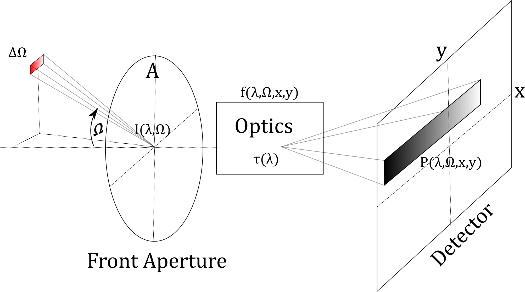
The incoming radiance, \(I(\lambda,\Omega)\), is incident upon the front aperture, propagates through the system and is distributed across the focal plane array surface by the optical system as a photon density function,
which is a continuous density function and has units \(\left[ photons\,sec^{-1}\,ster^{-1}\,nm^{-1}\,{\mu m}^{-2} \right]\): it represents the number of photons from direction \(\Omega\), wavelength \(\lambda\), striking the detector surface at location \((x,y)\). We have the following terms:
- \(A\) is the area of the front-end aperture in \(cm^2\).
- \(I(\lambda,\Omega)\) is the incoming radiance in direction \(\Omega\), wavelength \(\lambda\)
- \(\tau(\lambda)\) is an explicit, unit-less term that reflects the optical transmission of the optics. It can be folded into function \(f\) if desired.
- \(f(\lambda, \Omega, x, y )\) is a function that describes how signal from incoming
direction \(\Omega\) and wavelength \(\lambda\) is distributed across the detector surface. It is given in units of \({\mu m}^{-2}\)
The distribution, \(f(\lambda, \Omega, x, y )\), is typically more complicated than a simple one-to-one mapping as it accounts for the special physical properties of the optical systems we are trying to model. These systems typically include diffraction and interference. For example,
- a diffraction grating system (e.g. CATS, OSIRIS) images different wavelengths to different parts of the detector surface in one dimension.
- a spatial heterodyne system (e.g. SHOW) or Fourier transform spectrometer (e.g. LIFE) will distribute all incoming wavelengths across the entire detector surface in one direction.
- an imaging system (e.g. ALI) will, to first order, image the incomining solid angle to a corresponding area on the detector although chromatic aberrations may change this in second order.
The total photon signal, \(S\), incident upon an area, \(a\), is given by
which upon substitution for \(P\) from above becomes
or
where
In this latter notation we see that \(f^\prime(\lambda,\Omega, a)\) acts like a point spread function for the macroscopic area, \(a\), as it describes the contribution of each radiance at the front aperture to the total signal on the detector surface.