Instrument
Skimpy provides a high-level concept of an instrument which permits calculation of the radiance at the front aperture.
Each instrument in skimpy create a set of SpectralWindow objects that define the angular field
of view and wavelength pass-band defined at the instrument’s front aperture. The angular fields of view and wavelength
pass-bands are often chosen to match physical pixel properties on the detector plane but this is not required by skimpy
itself and users can create fields of view and wavelength pass-bands that do not correspond to any physical location on any
detector plane.
Each field of view within skimpy defines a array of lines of sight that span the angular field of view and are used within the skimpy radiative transfer model to calculate radiance across the field of view. Similarly each wavelength bandpass defines a range of wavelengths that span that range allows skimpy to calculate and account for signal variations (such as solar Fraunhofer structure) across the wavelength bandpass.
It is the responsibility of a user to create and configure an instrument class with the proper* skimpy* pixels. The instrument class must be
derived from Instrument. Individual fields of view and wavelength ranges are first created inside the instrument
and then skimpy pixels are created. For example:
class Test_Instrument( Instrument ):

def __init__(self):

    super().__init__( )

    # ---- setup the instantaneous field of views used by the pixels.

    fova = FOV_Rectangle( Hrange=(13, math.radians(0.0), math.radians(0.5)),             # Horizontal fov = 13 high resolution sub-divisions spanning 0.0 to 0.5 degrees
                          Vrange=(15, math.radians(0.0), math.radians(20.0 / 3600.0)))   # Vertical   fov = 15 high resolution sub-divisions spanning 0.0 to 20.0 degrees
                                                                                         # Creates a total of 13*15 = 195 lines of sight across the pixels rectangular area

    fovb = FOV_Rectangle( Hrange=(13, math.radians(0.7), math.radians(1.2)),             # Horizontal fov = 13 sub-divisions spanning 0.7 to 1.2 degrees
                          Vrange=(15, math.radians(0.2), math.radians(20.0 / 3600.0)))   # Vertical fov   = 15 sub-divisions spanning 0.0 to 20.0 degrees
                                                                                         # Creates a total of 13*15 = 195 lines of sight across the pixels rectangular area

    fovidx0= self.add_field_of_view( fova )                                              # Add the first rectangular field view to the instrument. Save the index
    fovidx1 = self.add_field_of_view( fovb )                                             # Add the second rectangular field of view to the instrument. Save the index

    # ---- setup the wavelength bandpass and range used by the pixel.

    wave0 = Wavelength_GaussianPSF( 30, 450.0, 0.3)                                     # spectral point spread function using 30 high resolution points, 450.0 nm with FWHM of 0.3 nm
    wave1 = Wavelength_GaussianPSF( 35, 452.0, 0.4)                                     # spectral point spread function using 35 high resolution points, 452.0 nm with FWHM of 0.3 nm
    wave2 = Wavelength_GaussianPSF(  1, 454.0, 0.5)                                     # spectral point spread function using  1 point, 454.0 nm with FWHM of 0.3 nm
                                                                                        # These three point spread functions may define up to 30 + 35 + 1 = 66 unique wavelengths (may be less if there is some overlap)

    wavidx0 = self.add_wavelength_range( wave0 )                                        # Add the spectral point spread function to the instrument. Save the index for later
    wavidx1 = self.add_wavelength_range( wave1 )                                        # Add the spectral point spread function to the instrument. Save the index for later
    wavidx2 = self.add_wavelength_range( wave2 )                                        # Add the spectral point spread function to the instrument. Save the index for later

    # ---- define the pixels used in this instrument in terms of the field of view and the wavelength bandpass.

    self.add_pixel( SpectralWindow( self, fovidx0, wavidx0) )                    # define the pixels used in the simulation. Pixels must use fields of view
    self.add_pixel( SpectralWindow( self, fovidx0, wavidx1) )                    # and spectral point spread functions which are already defined inside the instrument.
    self.add_pixel( SpectralWindow( self, fovidx0, wavidx2) )                    # Multiple pixels can use the same field of view.
    self.add_pixel( SpectralWindow( self, fovidx1, wavidx0) )                    # Multiple pixels can use the same spectral point spread function
    self.add_pixel( SpectralWindow( self, fovidx1, wavidx1) )                    # The radiative transfer code tries to ensure it does not repeat RT calculations
    self.add_pixel( SpectralWindow( self, fovidx1, wavidx2) )                    # although it must always calculate all unique wavelengths on all unique lines of sight
                                                                        # for this case that is around 195 lines of sight and 66 wavelengths.
Note that multiple pixels can share the same instance of a field of view object or wavelength bandpass object.
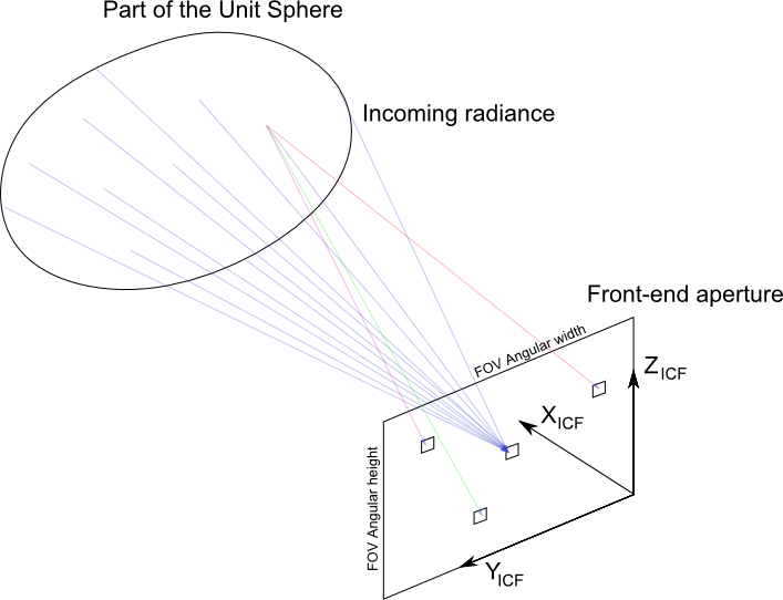
The complete angular field of view of the instrument (large rectangle) is divided into smaller solid angle regions for a simulation. Each small solid angle maps to one or more locations on the image plane. SpectralWindow objects are generated by combining one solid angle field of view with one wavelength bandpass object. The typical orientation of the Instrument Control Frame (ICF) is indicated.
Pixels
The SpectralWindow objects inside the user’s instrument class store the radiance signals
calculated by the skimpy radiative transfer engines. At the highest resolution the front-end radiance associated with the pixel
from scalar RTM calculations is a three dimensional array of the form,
where,
- \(\lambda\) is the wavelength dimension spanning all the wavelengths defined inside the wavelength bandpass of the pixel.
- \(\Omega_{LOS}\) is the field of view dimension. It indexes all of the lines of sight that span the instantaneous field of view of the pixel.
- \(N_{t}\) is the number of samples dimension. It spans all the locations and orientations of the instrument and platform used in the simulation.
The radiance array for polarized calculations is 4 dimensional, \(I\left[\lambda,\Omega_{LOS},N_{t},P \right]\), where \(P\) is the polarization dimension. It is 3 or 4 elements long and stores the Stokes vectors I,Q,U or I,Q,U,V.
Average Signals
Each SpectralWindow object internally stores the high resolution radiance signal and provides the user with the following integrated radiance related signals :
| Signal | Units | Symbol | Description. |
|---|---|---|---|
| radiance | Photons/cm2/nm/sec/ster | \(\bar{I}\) | the average radiance over the field of view and wavelength bandpass. |
| toa_albedo | /ster | \(\bar{\alpha}\) | top of the atmosphere albedo. Radiance divided by toa sun. |
| irradiance | Photons/cm2/sec | \(\bar{E}\) | the irradiance signal per unit area integrated over the field of view and wavelength bandpass window |
| photon flux | Photons/sec | \(\bar{P}\) | the photon flux integrated over the area of the front aperture, field of fov and wavelength bandpass |
We provide a brief theoretical basis for each of the averaged products. But first we provide a few clarifications,
The solid angle of the field of view of each pixel is given by \(\Omega_{fov}\) and we have the condition,
The spectral point spread function of each pixel, \(R(\lambda-\lambda_{0})\), is assumed to be a function of the difference of wavelength(e.g. Gaussian distribution). The spectral point spread function must be normalized such that,
The effective cross-sectionl area of the front end optics is given by, \(A\).
Average Radiance, \(\bar{I}\)
The spectrally and spatially average radiance, \(\bar{I}\), for the the pixel is given by the integral,
If the central wavelength, \(\lambda_0\), of the spectral point spread function does not change significantly across the field of view of a given pixel then we can simplify the equation to,
where \(\bar{\lambda_{0}}\) is the central wavelength of the pixel. This second, simplified form is the method currently implemented in skimpy as it allows the spectral point spread function to be represented as a function of wavelength only and can be represented by a one dimensional array.
The first, more general, equation requires the point spread function to be implemented as a two dimensional array and requires instrument specific knowledge that maps changes in angles to changes in wavelengths eg diffraction gratings. This calculation is not yet available in skimpy.
Average toa_albedo, \(\bar{\alpha}\)
The spectrally and spatially averaged toa_albedo, \(\bar{\alpha}\), is a similar calculation to the average radiance given by
which can also be reduced to a similar simpler form if the point spread function can be represented as function of wavelength only.
This second, simpler form is currently the only method implemented within skimpy.
Average Irradiance, \(\bar{E}\)
The spectrally averaged irradiance, \(\bar{E}\), is given by,
The integrals are numerically approximated with weighted sums in both wavelength and field of view but do not divide by the total solid angle of the
Average Photon Flux, \(\bar{P}\)
The total flux of photons through the front-end aperture in photons/sec is given by,
where
where \(A\) is the effective cross-sectional area of the front-end optics in cm2.
across the pixel is approximated by the weighted sum in wavelength and field of view. The weighted sum in wavelength include weights factors due to the spectral resolution of the instrument while field of view weights only account for the relative areas of the sub-divisions within the pixel.
The SpectralWindow object assigns a nominal wavelength and nominal line of sight to each sample/exposure in the observation set. The nominal wavelength is usually the center of the wavelength passband. The nominal line of sight is usually the center of the field of view. The SpectralWindow object provides the following ancillary information:
- the central line of sight of the field view in GEO coordinates
- the central wavelength of the wavelength bandpass
- the area of the front aperture optics
High resolution versions of the radiance and toa_albedo are also stored inside the SpectralWindow object, see below for more detail.
Number of Samples
Most instruments require a set of exposures or samples that follow an instrument specific observation policy to generate a data set appropriate for retrieval or analysis. For example, a limb viewing spectrograph must scan through a range of altitudes collecting exposures as it goes along. Within the Instrument model, the observation policy is simply represented as a set of, \(T\), samples containing the platform eciposition, orientation and time of measurement. The radiative transfer model calculates the pixel signal for each of the \(T\) samples applying the appropriate positional, pointing and time transformations as it does so.
Thus the signals actually stored in a SpectralWindow object are arrays that accomodate the number of samples in one observation set. If the radiative transfer model is scalar then the signals will be a 1-D array, \(I(T)\) of samples while polarized calculations will generate 2-D arrays of size \(I(T,4)\).
High Resolution Signals
The field of view and wavelength bandpass associated with each SpectralWindow object are often sub-divided into smaller sections to allow high resolution studies across both the field of view and the wavelength bandpass.
The pixel object automatically detects the sub-division and creates high resolution arrays to store both the radiance and toa_albedo returned from the call to the radiative transfer model at high resolution. The high resolution arrays are stored with two two extra leading dimensions for point spread wavelengths and instantaneous lines of sight, \(I(W,L,T)\) for scalar calculations or \(I(W,L,T,4)\) for polarizaed calculations.