LINEARCOMBO
A climatology that generates height profiles using a height dependent, linear combination of two climatologies. This is useful if one wishes to use one climatology in one height range and another climatology in another height range with a sensible transition region in between. If we let the first climatology generate value \(v_1(h)\) at a given height and the second climatology generate value \(v_2(h)\) at the same height then the LINEARCOMBO climatology will generate a value \(v(h)\) given by,
where \(f(h)\) is a height dependent function with a value ranging between 0 and 1. The user provides the height profile, \(f(h)\), as a linear piecewise function, \(f_{i}(h_i)\), consisting of \(N\) segments that span the height range of interest and,
\(f(h)\) is the factor applied to the first climatology and \(1-f(h)\) is applied to the second climatology. Values of \(f(h)\) above or below the height range of the piecewise function are truncated to the appropriate end value.
import numpy as np
import matplotlib.pyplot as plt
import sasktranif as skif
mjd = 52393.3792987115
labow = skif.ISKClimatology('O3LABOW') # The first climatology will be LABOW ozone
constant = skif.ISKClimatology('CONSTANTVALUE') # The second climatology witll be a constant value
constant.SetProperty('SetConstantValue', 4.0E12) # set the constant value to a fixed number
climate = skif.ISKClimatology('LINEARCOMBO') # generate the linear combo cliamtology
climate.SetProperty('SetFirstClimatology', labow) # set labow as the first claimatology
climate.SetProperty('SetSecondClimatology', constant) # set the the constant as the second climatology
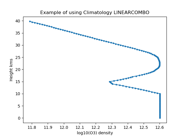
f = [ 10000.0, 0.0, 15000.0, 1.0] # Create the height profile of the linear combination
climate.SetProperty('SetHeightProfileCoeffsOfFirstClimatology', f ) # constant value below 10000, labow above 15000, linear in between
h = np.arange(0.0, 40000.0, 250.0)
ok,profile = climate.GetHeightProfile('SKCLIMATOLOGY_O3_CM3', [52.0, -106, 0.0, mjd], h)
plt.figure(1)
plt.plot( np.log10( profile), h/1000.0, '.-')
plt.xlabel( 'log10(O3) density' )
plt.ylabel('Height kms')
plt.title('Example of using Climatology LINEARCOMBO')
plt.show()
print('Done')
Supported Species
Only supports the species supported by both of the internal climatologies.
Cache Snapshot
The LINEARCOMBO climatology has no internal cache of its own. It uses the internal caches of the two compoent climatologies
Properties
- SetFirstClimatology(skClimatology climate)
Sets the first of the two climatologies used in the linear combination. The object passed in must represent an skClimatology object.
ISKClimatology.SetPropertyObject()
- SetSecondClimatology( skClimatology climate )
Sets the second of the two climatologies used in the linear combination. The object passed in must represent an skClimatology object.
ISKClimatology.SetPropertyObject()
- SetHeightProfileCoeffsOfFirstClimatology( Array linearpiecewise_profile )
Sets the piecewise linear height profile, \(f_i(h_i)\) of \(f\). The values of \(h_i\) and \(f_i\) are passed in as a single 1-D array where the order in memory is … \(h_i, f_i, h_{i+1}, f_{i+1}\)… . I.E. An array of height followed by value. The \(h_i\) are expressed as height in meters above sea level and must be in ascending order. The \(f_i\) are numbers between 0 and 1. The array passed in will be twice as big as the number of coefficients.
ISKClimatology.SetPropertyVector()